Vogel homebrew analog computer — Volume 7 — The valve sibling, the replications, and a bench reference

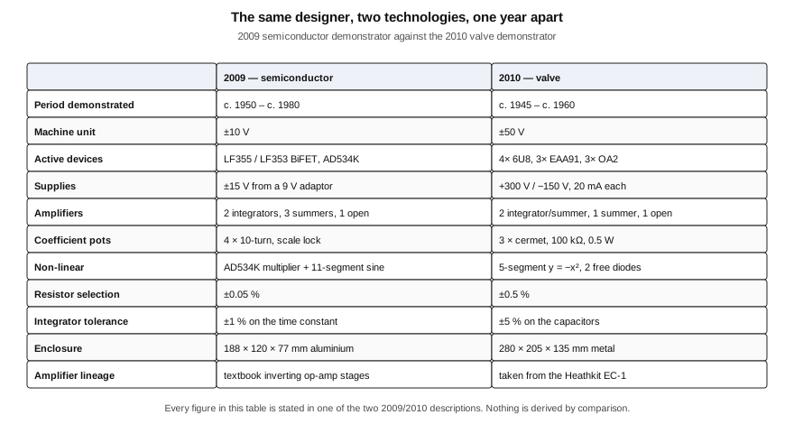
Figure 1 — The two machines set against each other. Every figure in the table is stated in one of the two descriptions; none is derived by comparison. Diagram authored for this dive.

7.1 About this Volume

Three subjects, in ascending order of practical usefulness.

First the 2010 valve demonstrator: the same designer’s account of building the same kind of machine in the technology of fifteen years earlier, which is interesting for what it reveals about the design decisions in the 2009 machine and for one unexpected disclosure about where its amplifier came from. Second the two documented replications, whose substitution lists are the nearest thing this design has to a sourcing guide. Third a consolidated bench reference drawn from all six preceding volumes.

Cross-references: Vol 1 §5 for the distinction between the machines; Vol 3 and Vol 4 for the 2009 machine’s elements, which this volume repeatedly sets the valve machine against; Vol 6 for the programs, which both machines share in substance.

---

7.2 The 2010 Valve Demonstrator

7.2.1 What It Is

Demonstrations-Analogrechner mit Röhren, F. Vogel, 21 August 2010, eight pages. Its opening sentence parallels the 2009 document’s exactly, with the period shifted:

“This small valve analog computer serves to demonstrate electronic analog computing technology as it was used from about 1945 to about 1960, and was then very rapidly displaced by transistor and semiconductor computers.”

Table 1 — What It Is

Parameter	Value
Valve complement	10 tubes: 4 × 6U8, 3 × EAA91, 3 × OA2
Supplies	+300 V at 20 mA, −150 V at 20 mA, stabilised
Machine unit	±50 V
Accuracy-relevant resistors	selected to ±0.5 %
Integrator capacitors	±5 %
Enclosure	metal, 280 × 205 × 135 mm (§1) or 133 mm (§4)
Computing elements	2 integrator/summers, 1 summer, 1 open amplifier/inverter
Coefficient potentiometers	3, single-turn cermet, 100 kΩ, 0.5 W
Function generator	1, for y = −x², five segments
Free diodes	2
References	+50.0 V and −50.0 V
Readout	moving-coil meter with address selector and range switch
Construction	two boards: amplifier board and power-supply board

Every specification is looser than the 2009 machine’s, in each case by roughly a factor of ten — ±0.5 % resistors against ±0.05 %, ±5 % capacitors against ±1 % time constants, ±0.5 V references against a REF01. That is not a worse machine so much as an honest one: it demonstrates the accuracy the technology of 1945–60 actually delivered, which is the point of building it.

Note — The two case-height figures, 135 mm in §1 and 133 mm in §4, are both in the same eight-page document. Neither can be preferred on the evidence held. See Vol 1 §7.

7.2.2 The Amplifier Came from the Heathkit EC-1

The most valuable sentence in the 2010 document is a disclosure that no other source in this hub provides:

“The circuit design of these amplifiers was taken from the analog computer EC-1, which was developed by the Heath Company as a training computer and came onto the market around 1960.”

Four identical computing amplifiers, built on the EC-1’s topology. The document then does something the Heathkit manual never does — it explains why the EC-1’s amplifier works as well as it does:

“It is of course not possible to build a high-quality DC amplifier with only one pentode-triode. Through a very skilful circuit design, however, Heath succeeded in optimising the properties with respect to gain factor, linearity and low output resistance so far that the amplifiers completely satisfy the requirements of a training or demonstration computer.”

The stages as described in the 2010 document:

Table 2 — The stages as described in the 2010 document

Feature	Description as given
Input stage	pentode with a very high anode resistor of 10 MΩ and a screen-grid voltage of only about 10 V
Coupling	second valve stage coupled to the first without a voltage divider
Gain boost	a small positive feedback through R15, 2.2 MΩ, to raise total gain to about 1000
Stability	a low-pass filter R14 / C11 added to stop that positive feedback causing oscillation, which “greatly reduces the cut-off frequency of the amplifiers — but for the intended application that is of no consequence”
Output stage	second valve as a cathode follower, giving very low output resistance
Level shift	because of the direct coupling the triode cathode sits far above zero, so it is shifted down by about 120 V by two neon lamps in series
Result	”very good linearity” across the normal ±50 V working range, from the measured gain diagram

Two of those entries deserve emphasis.

The positive feedback is a deliberate gain multiplier, not a fault. A small amount of regeneration through a 2.2 MΩ resistor raises the open-loop gain to about a thousand, at the cost of a stability margin that has to be bought back with an RC roll-off. That is a classic valve-era technique and it is stated here plainly, which is more than most period documentation does.

The neon-lamp level shifter is the cheapest possible solution to the hardest problem in direct-coupled valve design. Two glow lamps in series drop a fixed 120 V regardless of current — a zener diode before zener diodes were available at that voltage — and they cost a few pence each. The alternative, a resistive divider, would have thrown away most of the first stage’s gain, which is exactly what the document says the design avoids.

Note — This series makes no claim about whether the Heathkit EC-1’s own amplifier contains these features. The 2010 document says Vogel’s amplifier topology was taken from the EC-1 and then describes his implementation, including component designators (R14, R15, C11) that belong to his own schematic, not Heathkit’s. Anyone wanting to compare should read the two schematics side by side; the EC-1’s is held in this project, and Vogel’s is not.

7.2.3 The Four Amplifiers and Their Fixed Functions

As in the 2009 machine, the amplifiers have fixed functions rather than plug-in feedback. The assignment:

Table 3 — As in the 2009 machine, the amplifiers have fixed functions rather than plug-in feedback. The assignment

Amplifier	Function	Transfer function
A1, A2	integrator or summer, switch-selected	SUM: y = −(x₁ + x₂) · RUN: y = −(1/T)∫₀ᵗ(x₁ + x₂)dt − IC, T = 1 s · RES: y = −IC
A3	summer, three inputs	y = −(x₁ + x₂ + 2·x₃)
A4	open amplifier	y = −A·(x₁ + x₂), A ≈ 1000; SP input gives the summing point

Three differences from the 2009 machine are worth recording, because they change the programs.

A1 and A2 can be summers. The valve machine’s mode switch offers SUM in addition to RUN and RES, so an integrator not needed for integration can be pressed into service as a summer. That matters on a machine with only one dedicated summer, and it is a facility the 2009 machine does not have.

A3’s heavy input has a weight of 2, not 10. This single change propagates through the whole companion workbook: where the 2009 workbook’s §1.1 obtains y = −2x and y = −3.33x from its summer tricks, the valve workbook obtains y = −3x and y = −2.5x from the same techniques on a summer weighted differently.

Using A4 as an inverter has a precondition, and the document states it as a rule: “When used as an inverter the input SP must not be connected.” Tying the output back to x₂ makes a unity inverter; anything patched to the summing point at the same time defeats it.

7.2.4 The Function Generator: y = −x² by Divider

The valve machine’s diode function generator makes a different function by a different method, and the contrast with the 2009 sine generator is the single most instructive comparison between the two machines.

Table 4 — The Function Generator: y = −x² by Divider

	2009 machine	2010 machine
Function	sin x	y = −x²
Range	−1 ≤ x ≤ +1	0 ≤ x ≤ +1 (0 to +50 V)
Segments	11	5
Break points set by	selected zener diodes	divider resistors R82 – R89
Slopes set by	P12 – P17	P1 – P5
Stated maximum deviation	< 0.5 %	< 1 %
Range extension	not applicable	two free diodes and an inverter extend it to −1 ≤ x ≤ +1

The resistive-divider scheme is the conventional one described in Vol 4 §4.4 — eight tapped resistors fixing where each diode begins to conduct — and it is what a valve-era machine would actually have used. The five-segment approximation to a parabola over a single quadrant reaches 1 %, against eleven segments reaching 0.5 % on a full sine lobe; both are appropriate to their machines.

The two free diodes are a facility the 2009 machine provides differently. Where the semiconductor machine puts its spare diodes into a patch cord (Vol 2 §6), the valve machine brings two out to the programming field as elements in their own right. The effect is the same and the valve machine’s version is tidier; the 2009 machine’s diode cable is the cheaper answer on a panel with no room to spare.

7.2.5 Supply and Construction

The power supply is the place where the valve machine’s modest current demand pays off, and the document makes the reasoning explicit:

“Since the total current requirement of the four computing amplifiers is only about +15 mA and −20 mA, the voltage supply was built with three OA2 stabiliser tubes without additional series regulator valves.”

Three glow-discharge regulators and no series pass valve at all. On a machine drawing twenty milliamps, a shunt regulator is the regulator, and the whole apparatus of an error amplifier and a pass tube — which the EC-1 carries for its +300 V rail — becomes unnecessary. The same supply also produces the ±50 V references, which are generated by two selected zener diodes in series on each polarity, accurate to ±0.5 V.

The mechanical arrangement contains one detail worth repeating to anyone building valve equipment:

“The power-supply board is populated on both sides. All power resistors are mounted on the underside of the board and are cooled through the ventilation grille of the base plate. This prevents heating of the electrolytic capacitors on the upper side of the board.”

Power resistors below, electrolytics above, a vented base plate between them. It costs nothing at layout time and it is the difference between a supply that lasts and one that dries out its capacitors.

7.2.6 What Is Not Held

The 2010 document refers to “Schaltbild 1: Rechen-Verstärker”, “Schaltbild 2: Stromversorgung, Dioden-Funktionsgeber, freie Dioden, Koeffizienten-Potentiometer, Referenz-Spannungen, Anzeige-Instrument”, and component-placement plans for both boards. None of these is held in this project’s library. Everything above is therefore from prose, and no component-level walk of the valve machine is possible here in the way Vols 3 to 5 walk the semiconductor machine.

---

7.3 The RAR Workbook

The valve machine’s companion workbook is held: ten pages, the same seven-section structure, computing at ±50 V. Its content is close enough to the 2009 workbook that Vol 6 covers the substance for both, and the differences are exactly the ones the hardware forces:

Table 5 — The valve machine's companion workbook is held: ten pages, the same seven-section structure, computing at ±50 V. Its content is close enough to the 2009 workbook that Vol 6 covers the substance for both, and the differences are exactly the ones the hardware forces

Point	2009 workbook	RAR workbook
Machine unit	±10 V	±50 V
Summer trick results (§1.1)	y = −2x, −0.5x, −3.33x	y = −3x, −0.5x, −2.5x
Constant for integration	from a summer	from a coefficient potentiometer on the −1 reference
Non-linear section	multiplier: ×, ÷, x², √x	diode function generator: y = −x², quadratic equation
Trigonometric section	sin, cos, sin 2x	absent — the machine has no sine generator
Open-amplifier saturation	approx. ±14 V	approx. +120 V and −100 V
Undamped oscillator	C = 1 → 0.159 Hz; C = 10 → 1.59 Hz	C = 2 → 0.318 Hz
Readout	oscilloscope for fast programs	”the bipolar scale of the display instrument and the large integrator time constants allow direct observation of dynamic processes, even without an oscilloscope”

Two of those rows are worth a remark.

The valve machine’s open amplifier saturates asymmetrically, at about +120 V and −100 V — figures that sit far outside its ±50 V computing range in both directions and are not mirror images of each other. The comparator program therefore has to clip harder than the 2009 machine’s does, and the workbook’s conditioning chain limits the surviving polarity to −50 V with a coefficient potentiometer exactly as Vol 6 §5.1 describes.

The valve machine is designed to be watched on its own meter. That sentence about direct observation without an oscilloscope is the clearest statement in either document of what a demonstration computer is for. A ±50 V machine unit on a centre-zero meter with a ±100 scale gives a needle that swings across half the dial for a full-range variable, at a speed a person can follow.

Note — As Vol 1 §6 sets out, this project’s library catalogue attributes the RAR workbook to “Oliver Bach” on the strength of the PDF’s metadata. The content is the companion workbook to Vogel’s valve machine, in Vogel’s structure, and carries no by-line. This series treats the authorship as unresolved.

---

7.4 The Two Documented Replications

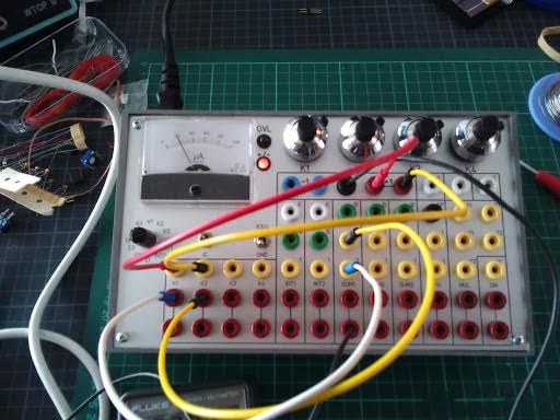
Figure 2 — The 2017 replication, patched and running. Photograph: “Coffee, bits and bikes”, 18 February 2017, CC BY-SA 3.0.

Neither replication is a Vogel machine, and both are labelled as replications wherever they appear in this series. They are valuable for one reason: each one records what its builder could not obtain, and what they did instead. That is the sourcing information the design itself never carried.

7.4.1 The 2010 Replication — analogmuseum.org

Built in March 2010 by Bernd Ulmann, on printed circuit boards donated by Dr. Vogel — which is the strongest evidence held that the 2009 design existed as a board run rather than as a one-off.

Table 6 — The 2010 Replication — analogmuseum.org

Original	Substituted	Consequence as stated by the builder
REF01 reference	LM317 regulating the positive machine unit	”cheap and imprecise”; “this made some small circuitry changes necessary”
LF355 / LF353	TL081 / TL082	the TL081 needs a negative bias for zero correction where the LF355 needs a positive one; rather than rework the circuit, “pins 1 and 5 of all TL 081” were bent up and the offset adjustment abandoned
AD534K	AD734	”pins 3, 4 and 5 must be tied to ground for proper operation in this context”
SMD resistors	axial resistors	”worked out quite well”

Three further build notes from the same account:

• The front panel is cut from printed-circuit-board material, and that material proved too thin to hold the ten-turn potentiometers — four spacers were made from an old front plate. Figure 3 of Vol 2 shows the result.
• The wiring between the patch board and the main board “took more time than expected”.
• The sine generator “was quite some work” — which is what seven interacting slope adjustments and ten selected zeners should be expected to cost, and which Vol 5 §8 is the reason for placing it last in any alignment.

The first row of that table is the consequential one. An LM317 is not a voltage reference, and the machine unit is the machine’s definition of the number one. Everything in Vol 3’s error budget — coefficients, initial conditions, constants — is a fraction of that voltage, so substituting a general-purpose regulator for a precision reference does not degrade one part of the machine; it degrades every number the machine produces. The builder says so in as many words (“cheap and imprecise”), and the substitution is presented in the source as a stopgap.

The second row is nearly as consequential and more subtle. Bending up the offset-null pins does not merely leave the amplifiers untrimmed — it leaves the integrators untrimmed, and an integrator’s offset integrates. A few millivolts of untrimmed offset on a 1 s time constant is a drift the operator will watch cross the meter.

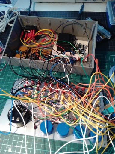
Figure 3 — The 2017 replication’s interior, showing the three-board arrangement its builder describes: the mains power supply on the white board, the “measuring card” in brown carrying the second schematic page plus the multiplier and sine generation, and the integrator capacitors and adders to the right. Photograph: “Coffee, bits and bikes”, CC BY-SA 3.0.

7.4.2 The 2017 Replication — “Coffee, bits and bikes”

Built between 2014 and 2017 from the published schematics, with no donated boards — the front panel was designed and sent for fabrication in 2014, and construction took “two weeks on several pcb pre-drilled boards” once the parts had been gathered.

Table 7 — The 2017 Replication — "Coffee, bits and bikes"

Original	Substituted	Reason given
DC/DC converter from a 9 V adaptor	mains transformer, rectifier, LM317 + LM337 at ±15 V	”I wanted a mains input and a linear regulator for each polarity”
LF355 / LF353	LF411 / LF412	not stated
Two polarity lamps	one bi-colour red / green LED	”with this I could save one extra hole in the front panel”
Eleven-segment diode sine generator	AD639 trigonometric function generator	”I couldn’t afford the space for the pots and diodes”
AD534K	AD534	obtained eventually; “the ones remaining in ebay are made of unobtanium”
Fixed integrator input resistors	potentiometers as input resistors	”so that I could adjust the time constants”
4 mm patching	2 mm plugs and sockets	implied by panel density

Two of those rows connect directly to findings in earlier volumes.

Replacing the diode ladder with an AD639 is the largest departure either builder made, and it is instructive about what the sine generator costs in real estate: ten selected zeners, six diodes, seven multi-turn potentiometers and two amplifier sections, all to do what one integrated circuit does. The builder’s reason is space, not accuracy. Anyone rebuilding this design for use rather than for authenticity should weigh the same trade; anyone rebuilding it to understand how period machines generated functions should build the ladder, because the ladder is the lesson.

Making the integrator input resistors adjustable is a direct response to the question Vol 3 §4 leaves open. With potentiometers in place of the fixed 966 kΩ and 96.6 kΩ networks, the time constant can be set to exactly 1.000 s against whatever the capacitor actually measures — which removes the whole question, and is what one would do having noticed that the published constants and the published resistor values do not agree.

7.4.3 What the Substitutions Tell a Builder

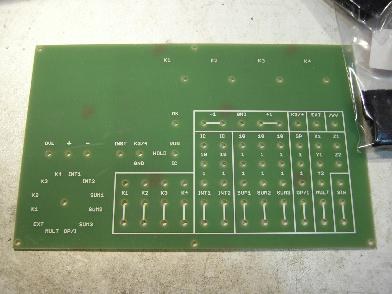
Figure 4 — The front panel before assembly, cut from circuit-board material. Roughly fifty patching holes plus the meter and potentiometer cut-outs; the material’s thinness was the one construction problem both accounts mention. Photograph: attributed to Bernd Ulmann / analogmuseum.org, March 2010.

Taking the two accounts together, the parts fall into three classes:

Table 8 — Taking the two accounts together, the parts fall into three classes

Class	Parts	Guidance from the accounts
Genuinely hard	AD534K	Neither builder obtained the K grade. One used an AD734, one waited and obtained a plain AD534, remarking on scarcity. Any four-quadrant multiplier of comparable accuracy will serve; the panel terminals are the device’s own pin names, so a substitution changes the patching.
Laborious rather than hard	the eleven-segment sine ladder	Ten selected zeners and seven interacting trimmers. One builder did it and called it “quite some work”; one avoided it with a single IC.
Freely substitutable	op-amps, converter, indicator LEDs, patch hardware	Both builders changed all four without apparent consequence. Any JFET-input amplifier of the era serves; a mains supply serves as well as the converter, at the cost of portability.
Do not substitute	the voltage reference	The one substitution a builder explicitly regretted in print. The machine unit is the machine’s definition of one.

Tip — The offset-null pin polarity caught one builder out and is the trap most likely to catch the next. The LF355’s null circuit returns its wiper to the positive rail; several otherwise-equivalent JFET amplifiers return theirs to the negative rail. A substitution that ignores this does not fail visibly — it simply leaves every amplifier untrimmed, and the integrators drifting.

---

7.5 Consolidated Bench Reference

Everything below is drawn from Vols 1 to 6 and refers to the 2009 semiconductor machine.

7.5.1 Terminal Map

Table 9 — Terminal Map

Terminals	Element	Terminals	Element
1 / 2 / 3 → 4	INT1: IC, ×10, ×1 → out	27 / 28 / 29 → 30	OP/I: SP, ×1, ×1 → out
8 / 9 / 10 → 11	INT2: IC, ×10, ×1 → out	31 / 32 / 33	MUL: X1, Y1, Y2
15 / 16 / 17 → 18	SUM1: ×10, ×1, ×1 → out	34 / 36 → 35	MUL: Z2, Z1 → out
19 / 20 / 21 → 22	SUM2: ×10, ×1, ×1 → out	39 → 40	SIN: x → out
23 / 24 / 25 → 26	SUM3: ×10, ×1, ×1 → out	47 / 48 / 49	+1, −1, ground
42 / 43 / 46	polarity POS, NEG; overload	44 / 45	selector wiper; triangle out

7.5.2 Element Transfer Functions

Table 10 — Element Transfer Functions

Element	Function	Range	Static error
Summer ×3	y = −(x₁ + x₂ + 10·x₃)	±1	≤ 0.1 %
Integrator ×2	y = −∫₀ᵗ(x₁ + 10·x₂)dt − IC	±1	T = 1 s / 0.1 s, ±1 %
Open amplifier	y = −A(x₁ + x₂), A > 3 × 10⁵	saturates ≈ ±14 V	—
Coefficient pot ×4	y = k·x, 0 ≤ k ≤ 1	±1	set in circuit
Multiplier	×, ÷, x², √x	see Vol 4 §3	0.2 – 0.3 %
Sine generator	y = sin x, x = φ/90°	±1	< 0.5 %
Triangle generator	±1 ramp	1.5 – 75 Hz	—

7.5.3 Operating Sequence

1. Connect the 9 V adaptor; switch on. No warm-up is required.
2. Patch the program completely, including every coefficient potentiometer, before setting any coefficient.
3. Select each potentiometer on the address selector and set its coefficient against an external DVM, reading the delivered voltage (Vol 3 §6).
4. Set the initial conditions with the mode switch at IC, reading each integrator output on the selector.
5. Switch to RUN.
6. Walk the address selector across every element in the program while it runs, watching the overload lamp (Vol 5 §6).
7. Use HOLD to freeze the solution for measurement; droop is about 6 mV per minute.
8. Return to IC through HOLD to re-run.

7.5.4 Indicator Meanings

Table 11 — Indicator Meanings

Indication	Means
Green / POS lamp	the selected variable is positive
Red / NEG lamp	the selected variable is negative
Overload lamp	the selected element exceeds ±1.03 machine units — not a machine-wide alarm
Needle pinned	the selected variable is beyond ±10 V, or the meter range is wrong
Both polarity lamps flickering	the variable is near zero; normal at a zero crossing

7.5.5 Troubleshooting Triage

Table 12 — Troubleshooting Triage

Symptom	First suspicion	See
Answer plausible but wrong	an intermediate variable saturated; walk the selector	Vol 6 §2.2
Coefficient delivers less than its dial	set out of circuit; the pot is loaded by 100 kΩ	Vol 3 §6
Integrator drifts with inputs grounded	offset trim P1 or P2	Vol 5 §8
Square-root program reads one diode drop high	read after the diode, not at terminal 35	Vol 4 §3.4
Division latches at a rail	the divisor crossed zero or went negative	Vol 4 §3.2
Open amplifier will not invert	something is patched to terminal 27	Vol 3 §5
Switching hash on every output	decoupling capacitors omitted or the converter unfiltered	Vol 5 §3
Solution runs 3 % fast or slow	the integrator time-constant question	Vol 3 §4
Oscillatory program decays when it should not	amplifier and capacitor losses; expected	Vol 6 §8.2

7.5.6 What the Held Record Does Not Contain

For completeness, gathered from all seven volumes:

• No parts list, board artwork or construction sequence for either machine.
• No schematics for the 2010 valve machine.
• No calibration or alignment procedure for either machine; sixteen of eighteen trimmers on the 2009 machine are unexplained.
• No dates of construction, quantities built, prices or service history.
• No specification for the integrating capacitors beyond “1 µF”.
• No explanation of the 966 kΩ / 96.6 kΩ integrator input networks.

---

7.6 Closing

The Vogel demonstration computers are not important machines. Nothing was computed on them that needed computing, they were built half a century after the technology they demonstrate had been superseded, and the number in existence is probably in single figures.

What makes them worth seven volumes is that they are the only machines in this hub for which the designer’s reasoning survives alongside the design. The EC-1 has an assembly manual that tells the reader which wire to solder next and never why. The TR-10 has a brochure that explains what its architecture achieves and never how. Here there is a complete schematic, a description that says which properties each part was chosen for, a workbook that publishes the machine’s own failure as its most important example, and a second machine built a year later in an obsolete technology purely to show what that technology could and could not do.

Read together, the two machines make an argument that no single machine could: that the difficulty in analog computing was never the arithmetic. Three summers and two integrators, in valves or in silicon, will solve a second-order differential equation. What costs the other half of the board — the reference that defines one, the selector that lets any node be read without disturbing it, the rectifier that lets a bipolar variable drive a unipolar needle, and the lamp that lights when an answer has quietly stopped being an answer — is everything required to make the result trustworthy. A demonstration computer small enough to hold makes that division visible in a way a room full of racks never could, which is presumably why it was built.