Vogel Homebrew · Volume 1
Vogel homebrew analog computer — Volume 1 — Overview & the documentary record
What the machine is, who designed it, the three separate machines that carry the name, and exactly which documents this series stands on
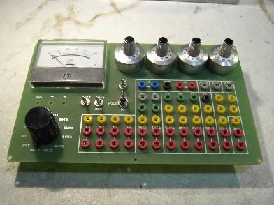
Figure 1 — A completed machine built to Dr. Vogel’s design, on boards he supplied. The instrument occupies a case 188 × 120 × 77 mm; everything the operator touches is on this one face. Photograph: attributed to Bernd Ulmann / analogmuseum.org, March 2010 — see photo_credits.txt for the basis of that attribution.
1.1 About This Volume
This volume establishes what the Vogel demonstration analog computer is, who built it, and — as prominently as the machine itself — which documents the rest of this series rests on and where they stop.
That second point is not a formality here, and it is not the same constraint as in the EAI PACE TR-10 series. The TR-10 problem was scarcity: a sales brochure and a procurement specification standing in for a manual that was never obtained. The Vogel problem is the opposite and rather more pleasant. A complete two-page schematic of every circuit in the machine is held, with designators and values, drawn by the designer. So is a nine-page description in his own words. So is an eighteen-page workbook of worked programs, with oscillograms. What is not held is anything a manufacturer would have produced — no production record, no serial numbers, no parts list, no board artwork, no revision history — because there was no manufacturer. This is one engineer’s machine, documented the way an engineer documents a machine for other engineers, and the gaps are exactly the ones that leaves.
The consequence for the reader is that this series can do something the TR-10 series could not: walk a signal from a patching socket, through a named resistor, into a named amplifier pin, and out again. Volumes 3 to 5 do that. It also means that where the schematic and the prose disagree — and they do, in two identified places — this series prints both and says which document each reading came from.
1.1.1 Depth-Index: The Seven-Volume Series
Table 1 — Depth-Index: The Seven-Volume Series
| Vol | Title | Primary content |
|---|---|---|
| 1 | Overview & the documentary record (this volume) | What the machine is, the designer, the three machines bearing the name, the sources and their limits, specifications quick-table |
| 2 | The console and the programming field | Enclosure, panel organisation, the terminal-by-terminal patch field map, the cable set, the operating controls, what is deliberately absent |
| 3 | The linear computing elements | Summers, integrators, the open amplifier, the coefficient potentiometers — schematic walk with designators, and the integrator time-constant question |
| 4 | The non-linear elements | The AD534K multiplier unit and its four modes; the eleven-segment sine diode function generator, breakpoint by breakpoint |
| 5 | Reference, supply, metering and monitoring | The REF01 reference chain, the DC/DC supply architecture, the precision rectifier and meter, the polarity and overload indicators, the triangle generator |
| 6 | Programming the machine | Machine units and scaling, and the workbook’s twenty worked programs re-derived and checked — including the one that returns a wrong answer on purpose |
| 7 | The valve sibling, the replications, and a bench reference | The 2010 vacuum-tube demonstrator, the RAR workbook, the two known replications with their substitution tables, and a consolidated reference |
Note — Cross-references appear throughout as “see Vol N §M”. Each volume is self-contained; this one assumes no other volume has been read.
1.2 What the Machine Is
1.2.1 A Demonstrator, Not a Teaching Kit and Not an Instrument
The 2009 machine is a miniature general-purpose electronic analog computer, built from discrete standard parts on a single double-sided board, housed in an aluminium case the size of a hardback book, and programmed by pushing 2 mm patch cords into a field of sockets on its front face.
Its own description states its purpose in the first sentence, and the phrasing is precise: it exists “to demonstrate electronic analog computing technology as it was used from approximately 1950 to approximately 1980, before being rapidly replaced by digital computers.” The complement of computing elements, it goes on, “has been tailored to these calculation examples.”
That is a different design brief from any of the commercial machines in this hub, and the difference runs all the way down into the circuitry. The Heathkit EC-1 was sold to teach analog computing to a student who would then move on to a real machine; its nine identical amplifiers are general-purpose and the user decides what each one becomes. The EAI PACE TR-10 was sold to solve an engineer’s actual differential equations; its capability is an inventory question, expandable by plugging in more modules. The Vogel demonstrator is aimed at neither. It is sized to a fixed, published set of twenty worked problems, and every element in it exists because one of those problems needs it. There are three summers because the hardest linear program in the workbook needs three. There is one multiplier and one sine generator because no program needs two.
This has a consequence worth stating at the outset, because it governs how the rest of the series reads the hardware: the machine is not expandable and is not meant to be. There are no spare positions, no module format, no bus. Its amplifiers are not identical to one another and cannot be repurposed — a summer is permanently a summer, wired with its feedback resistor on the board, and an integrator is permanently an integrator, wired with its capacitor on the board. Only one amplifier, the open amplifier, has no feedback element and can be made into anything; Vol 3 §5 treats it as the exception it is.
1.2.2 Where It Sits Among This Hub’s Machines
Table 2 — Where It Sits Among This Hub's Machines
| Heathkit EC-1 | EAI PACE TR-10 | Vogel 2009 | Vogel 2010 (valve) | |
|---|---|---|---|---|
| Era of manufacture | 1960 | c. 1960–1966 | 2009 | 2010 |
| Technology | vacuum tube | transistor | BiFET monolithic op-amp | vacuum tube |
| Machine unit | ±60 V | ±10 V | ±10 V | ±50 V |
| Computing amplifiers | 9, identical, general-purpose | up to 20, plug-in modules | 6, function-fixed | 4, function-fixed |
| Coefficient potentiometers | 5 | up to 24 | 4 | 3 |
| Multiplier | none | quarter-square, plug-in | one, AD534K | none |
| Function generator | none as standard | plug-in DFGs | one, sine, 11 segments | one, y = −x², 5 segments |
| Repetitive operation | yes, 0.1–15 c/s | yes, 20–500 ms | no | no |
| Supply | mains, ~100 W | mains, under 50 W | 9 V adaptor, ~1.8 W | mains, +300 / −150 V |
| Enclosure | 19¾ × 11½ × 15 in | 16 × 24 × 15 in | 188 × 120 × 77 mm | 280 × 205 × 135 mm |
Two rows in that table carry most of the argument. The power row is the headline difference of the modern machine: a general-purpose analog computer that runs all day off a 9 V wall adaptor at under two watts, where the EC-1 needs a hundred. The repetitive operation row is the deliberate sacrifice that makes the rest of it fit, and the 2009 description says so plainly rather than leaving it to be discovered: “A repetitive integrator control is not provided for this simple demonstration computer.” Vol 2 §6 sets out what that costs the operator and what is used instead.
1.2.3 What the Machine Does, in One Paragraph
A variable in the problem is a voltage, scaled so that the extremes of its range fall at ±10 V, which the machine calls ±1 machine unit. An operational amplifier with resistors from its inputs to its summing junction and a resistor in its feedback path forms the negated weighted sum of those inputs; the same amplifier with a capacitor in feedback instead forms the negated integral with respect to time. A ten-turn potentiometer across the reference multiplies a voltage by a constant between zero and one. A four-quadrant multiplier forms a product. A ladder of zener-defined breakpoints bends a straight line into a sine. Patch these together in the shape of a differential equation and, from the moment the integrator switch moves from IC to RUN, every voltage in the machine evolves exactly as the equation’s variables do — continuously, in parallel, in real time. Vol 6 develops this properly, from machine units upward.
1.3 The Designer
The documents are signed F. Vogel and dated. The only substantial biographical source held here is a doctoral dissertation, and it is worth a paragraph because it explains the machines rather than merely dating their author.
Dipl.-Ing. Fritz Vogel, of Bruck an der Leitha, submitted Ein elektronischer Koordinatenwandler ohne Diodennetzwerke und seine Anwendung bei der Messwertverarbeitung mechanischer Größen — “An electronic coordinate converter without diode networks, and its application in the processing of mechanical measured quantities” — to the Technische Universität Wien in September 1977. The work designs an analog circuit that converts Cartesian coordinates to polar in real time, replacing the conventional diode function network with an approximation to the arctangent built from an exponential characteristic. Its stated design requirements read, thirty-two years early, like a specification for the demonstration computer:
Table 3 — Dipl.-Ing. Fritz Vogel, of Bruck an der Leitha, submitted Ein elektronischer Koordinatenwandler ohne Diodennetzwerke und seine Anwendung bei der Messwertverarbeitung mechanischer Größen — "An electronic coordinate converter without diode networks, and its application in the processing of mechanical measured quantities" — to the Technische Universität Wien in September 1977. The work designs an analog circuit that converts Cartesian coordinates to polar in real time, replacing the conventional diode function network with an approximation to the arctangent built from an exponential characteristic. Its stated design requirements read, thirty-two years early, like a specification for the demonstration computer
| Dissertation requirement (1977) | Echo in the 2009 machine |
|---|---|
| Input signals available “in the range of ±10 V” | Machine unit is ±10 V |
| Output “also in the range of ±10 V” for oscilloscope or tape recording | Every computing element output is ±10 V, with an oscilloscope-compatible readout path |
| ”Maximum error should not exceed 1 % of the full scale value” | Summers ≤ 0.1 %, multiplier ≤ 0.3 %, sine generator < 0.5 % |
| Must “operate in real time” | Parallel, continuous solution; no repetitive mode needed |
| Operation “as simple as possible and without individual adjustment” | Coefficients set against an internal +10.00 V reference and an external DVM |
| ”Simple monitoring control of the computer must be possible” | Address selector, polarity indicator and overload lamp |
The dissertation’s application chapters are on acceleration measurement of a body with three degrees of freedom, and on biaxial stress analysis of a mechanically loaded body — measurement engineering, not computing for its own sake. The demonstration computers are the work of someone who used analog computation as a professional instrument before building a machine to explain it.
Note — The dissertation is held as a scanned document and its translation was produced by machine. Proper names in it — supervisors, institute titles — are exactly the material such a pipeline degrades, and none is repeated here. The author’s own name, degree, institution and date appear on the title page in several forms and are safe.
1.4 The Three Machines That Carry the Name
A reader arriving from a web search will find the name “Vogel analog computer” attached to at least three different pieces of hardware, and the sources held here describe all three. Conflating them is the most likely way to go wrong on this subject.
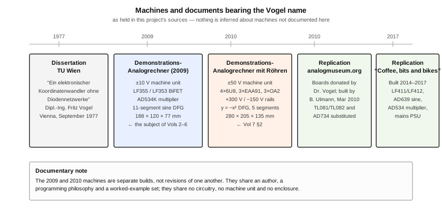
Figure 2 — What each document in this project’s sources actually describes. Diagram authored for this dive; every figure on it is stated in one of the held documents.
Table 4 — The Three Machines That Carry the Name
| Demonstrations-Analogrechner | Demonstrations-Analogrechner mit Röhren | |
|---|---|---|
| Document | F. Vogel, 9 pp., 06.05.2009 | F. Vogel, 8 pp., 21.08.2010 |
| Technology | BiFET monolithic op-amps | 10 vacuum tubes |
| Machine unit | ±10 V | ±50 V |
| Demonstrates the period | c. 1950 – c. 1980 | c. 1945 – c. 1960 |
| Schematic held here | yes, 2 pages, complete | no — the sheets are referenced but not held |
| Companion workbook held | yes, 18 pp., 20 examples | yes, 10 pp., as “Rechenbuch 1” |
These are separate builds, not revisions of one another. They share a designer, a programming philosophy and a nearly identical worked-example set, and they share no circuitry, no machine unit, no enclosure and no amplifier. Volumes 2 to 6 of this series are about the 2009 semiconductor machine, because that is the machine whose schematic is held. The 2010 valve machine gets Vol 7 §2, at the depth its thinner record supports.
The third thing bearing the name is not a Vogel machine at all: it is a replication. At least two are documented. Bernd Ulmann built one at analogmuseum.org in March 2010 from a set of printed circuit boards Dr. Vogel donated; an anonymous author of the weblog Coffee, bits and bikes built another between 2014 and 2017 from the published schematics. Both substituted parts, and both said which — Vol 7 §4 tabulates the substitutions, because they are the nearest thing to a sourcing guide this design has. Photographs of both appear in this series and are labelled as replications wherever they do.
1.5 The Documentary Record
1.5.1 The Five Primary Sources
Everything asserted in this series traces to one of the following.
Table 5 — The Five Primary Sources
| Source | What it is | Character |
|---|---|---|
| ”Demonstrations-Analogrechner”, F. Vogel, 06.05.2009 | 9-page German technical description of the ±10 V machine: overview, panel key, element-by-element specifications, programming, mechanical construction | The designer describing his own finished machine. Specific, numerate, and free of sales language. The primary source for every performance figure in Vols 2–5. |
The schematic sheet (held as Vogel - Demo Schematic.pdf, identically as _info/Misc Docs/vogel_schaltplan.pdf) | 2 pages. Page 1: the two integrators, three summers, open amplifier, multiplier, sine generator. Page 2: DC/DC converter, triangle generator, reference, coefficient potentiometers, address selector, precision rectifier, polarity and overload indicators | Complete at component level, with designators, values, IC types, pin numbers and every patch-field terminal numbered 1–49. This is the document that makes Vols 3–5 possible. |
| ”Rechenbeispiele” / calculation examples | 18-page workbook: 20 worked programs in seven sections, each with circuit, derivation and oscillogram | The machine’s reason for existing. Vol 6 works through it. |
| ”Demonstrations-Analogrechner mit Röhren”, F. Vogel, 21.08.2010 | 8-page description of the valve machine, same structure as the 2009 document | Detailed on the amplifier and supply; its schematics are referred to as “Schaltbild 1/2” but are not held here. |
| ”Rechenbeispiele für den RAR Analogrechner — Rechenbuch 1” | 10-page workbook for the ±50 V machine | Content-wise a sibling of the 2009 workbook. See the authorship note below. |
Two secondary sources are used, always labelled: the analogmuseum.org build page of 29 March 2010, and the Coffee, bits and bikes post of 18 February 2017. Both describe replications, not the original.
Note on the RAR workbook’s authorship — this project’s library catalogue records that document as “created in 2010 by Oliver Bach”. That attribution comes from the PDF’s own metadata, which on a document of this kind commonly records whoever operated the scanner or the layout tool rather than the author. The content is the companion workbook to Vogel’s ±50 V valve machine, in Vogel’s structure and register, and no by-line appears in the text. This series therefore treats the authorship as unresolved rather than adopting the metadata reading.
1.5.2 What Is Not Held
Stated plainly, because several of these would otherwise be assumed:
- No parts list or bill of materials. The schematic names every part; nobody ever wrote down where to buy them. Vol 7 §4 assembles what can be assembled from the two replication accounts.
- No board artwork or layout drawing for the 2009 machine. The description gives the board’s outline dimensions — 105 × 88 mm, populated on both sides — and a photograph shows its component side, and that is the whole of the record.
- No schematics for the 2010 valve machine. The 2010 text refers to “Schaltbild 1: Rechen-Verstärker” and “Schaltbild 2: Stromversorgung …”, and to board layout plans for both boards. They existed. They are not in this project’s library. Vol 7 §2 therefore describes the valve machine from its prose only, and says so.
- No calibration or alignment procedure. Seventeen trimmer potentiometers are drawn on the schematic, and the text explains what four of them are for. What the rest are set to, in what order, against what, is not documented. Vol 5 §7 reconstructs what can be reconstructed and labels it as reconstruction.
- No dates of construction, quantities built, or disposition. The documents are dated; the machines are not.
- No failure or service history. Nothing in the held record says what wears out.
1.6 Specifications Quick-Table
Every figure below is stated in the 2009 description or read off the schematic sheet. Nothing is derived or estimated.
1.6.1 The Machine
Table 6 — The Machine
| Parameter | Value | Source |
|---|---|---|
| Machine unit | ±10 V = ±1 | 2009 description §1 |
| Enclosure | aluminium, 188 × 120 × 77 mm | §1, §5 |
| Circuit board | 105 × 88 mm, populated both sides | §5 |
| External supply | 9 V DC / 1200 mA plug adaptor | §1, §3.12 |
| Internal rails | ±15 V, stabilised to ±0.5 %, from a DC/DC converter | §3.12 |
| Total power consumption | approximately 1.8 W | §3.12 |
| Op-amp technology | BiFET; input resistance 10¹² Ω, open-loop gain > 3 × 10⁵, offset typically 5 mV | §1 |
| Accuracy-relevant resistors | selected to ±0.05 % | §1 |
| Integrator time-constant tolerance | ±1 % | §1 |
1.6.2 The Computing Elements
Table 7 — The Computing Elements
| Element | Count | Transfer function | Stated static accuracy |
|---|---|---|---|
| Summer | 3 | y = −(x₁ + x₂ + 10·x₃) | ≤ 0.1 % error |
| Integrator | 2 | y = −∫₀ᵗ(x₁ + 10·x₂)dt − IC | time constants 1 s and 0.1 s, ±1 % |
| Open amplifier / inverter | 1 | y = −A(x₁ + x₂), A > 300 000 | — |
| Coefficient potentiometer | 4 | y = k·x, 0 ≤ k ≤ 1 | 10-turn, lockable dial |
| Multiplier unit | 1 | multiply / divide / square / square-root | 0.2 % / 0.3 % / 0.2 % / 0.2 % |
| Sine function generator | 1 | y = sin x for −1 ≤ x ≤ +1 | < 0.5 % departure, 11 segments |
1.6.3 Auxiliary Facilities
Table 8 — Auxiliary Facilities
| Facility | Specification | Source |
|---|---|---|
| Reference voltages | +10.00 V and −10.00 V, calibratable | §3.7 |
| Panel meter | ±10 V, accuracy class 2.5, defeatable | §3.8 |
| External DVM output | rear-panel sockets, parallel to the meter | §3.8 |
| Address selector | 12 positions, last selects a panel input socket | §3.9 |
| Overload indicator | thresholds ±10.3 V (±1.03 machine units), red LED | §3.10 |
| Triangle generator | ±10 V, 1.5 Hz to 75 Hz, side-mounted multi-turn control | §3.11 |
| Integrator modes | RUN, HOLD, IC; HOLD droop ≈ 6 mV per minute | §3.2 |
| Repetitive operation | none | §3.2 |
1.6.4 The Semiconductor Complement, as Drawn
Table 9 — The Semiconductor Complement, as Drawn
| Designator | Device | Function |
|---|---|---|
| IC1, IC2 | LF355 | Integrators 1 and 2 |
| IC3, IC4, IC5 | LF355 | Summers 1, 2 and 3 |
| IC6 | LF355 | Open amplifier / inverter |
| IC7 | AD534K | Multiplier unit |
| IC8 | marked LM353 on the sheet | Sine function generator, both sections |
| IC9 | LF353 | Triangle generator |
| IC10 | LF353 | Precision rectifier for the meter |
| IC11 | LF353 | Address-selector buffer and polarity comparator |
| IC12 | LM1458 | Overload window comparator |
| IC13 | REF01 | Precision voltage reference |
| IC14 | LF353 | Reference buffer / inverter |
| DC1 | TEN 3-1223 | 9 V to ±15 V DC/DC converter |
1.7 Where the Sources Disagree
Three divergences were identified while preparing this series. None is large, and all three are recorded here so that no later volume has to smooth over them.
Table 10 — Where the Sources Disagree
| Point | Reading A | Reading B | Comment |
|---|---|---|---|
| IC8’s type | The schematic sheet letters it LM353 | Every other dual on the same sheet — IC9, IC10, IC11, IC14 — is lettered LF353, and the machine is described as BiFET throughout | Almost certainly a slip of the pen for LF353, but the sheet says what it says. Vol 4 §4 uses “the device the sheet letters LM353” and notes the reading. |
| Open-amplifier terminal 27 | The schematic sheet prints the weight glyph “10” beside it | The front-panel artwork prints “SP” at the head of that column, and the 2009 text §3.3 describes the summing point as an accessible input | The terminal has no series resistor at all — a bare wire to the summing junction, which cannot carry a weight of 10 or of anything else. The panel and the text agree; the schematic glyph is an error. |
| Valve-machine case height | §1 of the 2010 document: 280 × 205 × 135 mm | §4 of the same document: 280 × 205 × 133 mm | A two-millimetre disagreement inside one document. Neither reading can be preferred on evidence. |
A fourth item is not a disagreement between sources but between the schematic and arithmetic, and it is the most interesting single finding in this series: the integrator input networks do not come to the round numbers the text implies. The weight-1 input is 910 kΩ + 56 kΩ = 966 kΩ, and the weight-10 input is 91 kΩ + 5.6 kΩ = 96.6 kΩ. Against a nominal 1 µF that is 0.966 s and 0.0966 s, not the 1 s and 0.1 s the description states, and the shortfall is 3.4 % against a claimed ±1 % tolerance. Vol 3 §4 sets out the two readings that could resolve it and declines to choose between them on the evidence held.
1.8 What Is Not Known
- Whether more than one 2009 machine was built. Dr. Vogel donated a set of boards to at least one replicator, which implies a run of boards, but no quantity appears anywhere.
- The integrating capacitor’s actual value and type. The schematic says “1 µF” and nothing else — no dielectric, no tolerance. Given that the description claims ±1 % time constants and the input resistors are selected to ±0.05 %, the capacitor is the constraint; but its specification is not held.
- What sixteen of the eighteen internal trimmers are set to. The sheet carries eighteen preset adjustments — six amplifier offset trims, seven shaping the sine generator, two on the reference, one on the meter and two on the triangle generator — and the held sources explain two of them. No calibration or alignment procedure for this machine exists in the record. Vol 5 §8 takes the census and reconstructs what can be reconstructed.
- Why the panel meter reads through a precision rectifier. The circuit is unambiguous — IC10 with matched 100 kΩ resistors and two diodes — but a class 2.5 movement does not need a precision rectifier’s accuracy. Vol 5 §5 offers the most economical explanation and labels it as inference.
- The designer’s intent for the machine’s afterlife. That the boards were donated and the documents published is the whole of the record.
1.9 Why the Machine Matters
Three reasons, in ascending order of durability.
It is the only machine in this hub whose schematic is complete and whose author is reachable in the text. For the EC-1 there is a manual but no designer’s voice; for the TR-10 there is a brochure and no schematic at all. Here there is a designer explaining, circuit by circuit, why each element is the way it is — including the places where he chose to leave something out. That makes it the best available worked example of analog computer design decisions, as distinct from analog computer operation.
It demonstrates that the hard part was never the amplifier. Six of the twelve integrated circuits in this machine do no computing at all. They are reference, metering, rectification, polarity, overload and stimulus. The computing elements — three summers and two integrators — are six op-amps and a handful of selected resistors, and any competent engineer could throw them together in an afternoon. What takes the other half of the board is everything needed to make the answer readable and trustworthy: a stable unity to scale against, a way to look at any node without patching, and a lamp that lights when a result has quietly stopped meaning anything. That division of effort is the honest lesson of analog computing, and a machine this small makes it visible in a way a room-sized installation never could.
It is a complete, buildable design in the public record. A reader with this schematic, the parts list Vol 7 assembles, and two weekends can have a working general-purpose analog computer on the bench — one that solves second-order differential equations in real time, to a tenth of a percent, off a wall adaptor. Very few machines documented in this hub can still be said to be available in that sense. This one can.
1.10 What Comes Next
Vol 2 opens the console: the panel organisation, the programming field terminal by terminal against the schematic’s own numbering, the four cable types, the operating controls, and the two facilities the machine deliberately does without. Vol 3 takes the linear computing elements one at a time with the schematic open. Vol 4 does the same for the multiplier and the sine generator. Vol 5 covers everything that is not computing — reference, supply, metering, monitoring and stimulus. Vol 6 is the programming volume and works through the twenty published examples. Vol 7 turns to the valve sibling, the two replications and their part substitutions, and closes with a consolidated bench reference.
Comments (0)