Vogel homebrew analog computer — Volume 2 — The console and the programming field

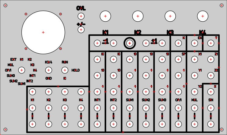
Figure 1 — The panel artwork, which is the authoritative statement of what each socket is called. Column names run across the bottom — K1 to K4, INT1, INT2, SUM1 to SUM3, OP/I, MUL, SIN — with the weight or terminal name printed beside each socket. Provenance: held in this repository; attributed to the “Coffee, bits and bikes” replication of 2017 (CC BY-SA 3.0), though it may be the designer’s own artwork. This could not be confirmed — see photo_credits.txt.

2.1 About this Volume

Volume 1 established what the machine is. This volume describes how it is put together and how the operator meets it: the enclosure and the single board inside it, the organisation of the front panel, the programming field socket by socket against the schematic’s own terminal numbers, the four kinds of patch cable, the operating controls, and — at the end — the two capabilities the design leaves out on purpose.

Everything here is drawn from two documents: F. Vogel, Demonstrations-Analogrechner, 06.05.2009, and the two-page schematic sheet. Where the panel artwork is used as evidence it is named as such, because on one terminal it settles a question the schematic gets wrong.

Cross-references: Vol 1 for sources and specifications; Vol 3 for what lies behind each computing column; Vol 5 for the meter, reference and monitoring circuits the panel controls reach; Vol 6 for the programs that fill this field with patch cords.

---

2.2 The Enclosure and What Is Inside It

The machine is built into an aluminium case measuring 188 × 120 × 77 mm — roughly the footprint of a hardback novel and about three times its thickness. Everything the operator interacts with is on the top face, which the description calls the front. The rear carries two sets of sockets: one for the 9 V DC plug adaptor, one for an external digital voltmeter. The right-hand side of the case carries a single multi-turn control, which sets the triangle generator’s frequency; that control is placed on the side rather than the face because it is a stimulus setting rather than a programming one, and it is set once for a run.

Inside is one board, 105 × 88 mm, populated on both sides, carrying every computing element, every auxiliary circuit and the power converter. There is no motherboard, no backplane, no module format and no second card. This is the structural expression of the design brief stated in Vol 1 §2: a machine sized to a fixed set of problems does not need to be able to become a different machine, and a machine that cannot become a different machine does not need the mechanical apparatus of expansion.

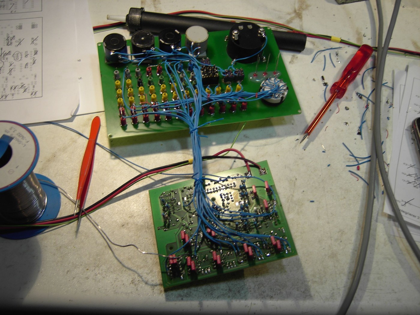
Figure 2 — The two halves during assembly of a machine built to this design: the patch-panel board with its sockets fitted, and the main board, joined by the harness that carries every signal between them. The single-board figure quoted in the description counts the main board; the patching field is a separate piece of board carrying the sockets. Photograph: attributed to Bernd Ulmann / analogmuseum.org, March 2010.

Two points follow from the photograph that the prose does not make explicit. First, the harness between the two boards is the machine’s only significant wiring, and it is substantial — roughly fifty conductors, one per terminal. Second, the patch field is a board, not a panel with sockets pushed through it, which is why the sockets sit in machined rows with no visible hardware. One replication account records that circuit-board material proved too thin to carry the ten-turn potentiometers, and that spacers had to be improvised; a builder working from this design should expect to solve that problem.

---

2.3 The Front Panel: The Designer’s Own Key

The 2009 description numbers the operating controls 1 to 8 and letters the programming field A to K. That key is reproduced here verbatim in translation, because every later reference in the source documents uses it.

Table 1 — The Front Panel: The Designer's Own Key

No.	Control	Treated in
1	Power switch	this volume §6
2	Display instrument (panel meter)	Vol 5 §5
3	Address selector switch	Vol 5 §6
4	Overload indicator	Vol 5 §4
5	Polarity indicator	Vol 5 §4
6	Switch for the display instrument	Vol 5 §5
7	Changeover switch for potentiometers K3 / K4	this volume §5
8	Integrator control (RUN / HOLD / IC)	Vol 3 §4

Table 2 — The Front Panel: The Designer's Own Key

Letter	Programming-field group	Treated in
A	Coefficient potentiometers	Vol 3 §6
B	Integrators	Vol 3 §4
C	Summers	Vol 3 §3
D	Open amplifier / inverter	Vol 3 §5
E	Multiplier unit	Vol 4 §2
F	Function generator for the sine function	Vol 4 §3
G	Reference voltages	Vol 5 §2
H	Base point for potentiometers K3 / K4	this volume §5
J	External input for the display instrument	Vol 5 §6
K	Triangle voltage generator	Vol 5 §7

Note — The panel diagram in the 2009 description also carries a callout numbered 9, for which the key gives no entry. The most economical reading is that it marks the triangle generator’s frequency control, which §3.11 of the same document places “on the right side of the computer case” and which would otherwise appear in no illustration. That is inference, not evidence.

The division embodied in those two lists is the important thing about this panel and is worth naming. Numbered items are things the operator sets or reads; lettered items are things the operator patches. No element appears in both lists. There is no control that alters the behaviour of a computing element from the front panel — no gain switch, no range switch, no time-scale selector. Everything a program needs is expressed in patch cords, and the numbered controls exist entirely to run the machine and to look at it. The one apparent exception, the integrator control at 8, proves the rule: it moves all integrators together and is the machine’s mode switch, not a per-element setting.

---

2.4 The Programming Field, Terminal by Terminal

The schematic sheet numbers every patching terminal in the machine. Those numbers do not appear on the panel — the operator sees column names and weights — but they are how the schematic and this series refer to a socket unambiguously.

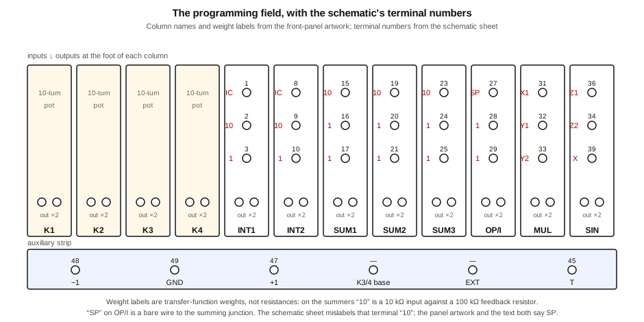
Figure 3 — The programming field, with column names and weight labels from the panel artwork and terminal numbers from the schematic sheet. Diagram authored for this dive.

2.4.1 The Full Terminal List

Table 3 — The Full Terminal List

Terminals	Belong to	Function
1, 2, 3	INT1	IC input; weight-10 input; weight-1 input
4	INT1	output (doubled socket)
5, 6, 7	S2A	contacts of the integrator-control switch, section A
8, 9, 10	INT2	IC input; weight-10 input; weight-1 input
11	INT2	output (doubled socket)
12, 13, 14	S2B	contacts of the integrator-control switch, section B
15, 16, 17	SUM1	weight-10 input; two weight-1 inputs
18	SUM1	output
19, 20, 21	SUM2	weight-10 input; two weight-1 inputs
22	SUM2	output
23, 24, 25	SUM3	weight-10 input; two weight-1 inputs
26	SUM3	output
27, 28, 29	OP/I	summing point (direct); two weight-1 inputs
30	OP/I	output
31, 32, 33	MUL	X1; Y1; Y2
34, 36	MUL	Z2; Z1
35	MUL	output
39	SIN	x input to the sine generator
40	SIN	output
41	metering	meter / rectifier node
42, 43	indicators	polarity lamps LD2 (positive) and LD3 (negative)
44	metering	address-selector wiper, and the external-DVM tap
45	K	triangle generator output
46	indicators	overload lamp LD1
47, 48, 49	G	+1 reference (+10.00 V); −1 reference (−10.00 V); ground

Note — The numbering as held runs to 49. Terminals 37 and 38 could not be located anywhere on the sheet at the resolution available, and the coefficient-potentiometer sockets K1 to K4 are drawn without terminal numbers at all. Both gaps are in the record, not in this transcription.

2.4.2 The Column Discipline

Every computing column is laid out identically: three input sockets in a vertical stack, a doubled output socket below. The label beside each input is its weight; the label below the column is its name. Once that pattern is read, the field needs no legend — an operator who knows the machine has three summers knows exactly where six of its nine input sockets are, and what each does.

Two consequences of the doubled output socket are worth stating, because the description mentions the feature only in passing and it changes how programs are patched. Every output is a two-socket bus. A variable that has to reach two places — and in a second-order program almost every variable does — is taken twice from its source rather than joined at its destination. There is no tie-point panel on this machine and no ground of convenience; fan-out is a property of the output, not a separate facility. And because two cords at an output are electrically parallel, the operator can trace a program by following cords outward from each column rather than inward, which is a materially easier way to check a patch.

2.4.3 Reading a Weight Label

A weight label is a transfer-function weight, not a resistance, and conflating the two is the commonest way to mis-read this panel. On the summers, “10” is a 10 kΩ input resistor working against a 100 kΩ feedback resistor, giving a gain of ten; “1” is a 100 kΩ input against the same 100 kΩ feedback, giving a gain of one. On the integrators the same labels mean something arithmetically parallel but physically different: the weight-10 input has roughly a tenth the resistance of the weight-1 input, so it charges the same capacitor ten times as fast, and the integration time constant is 0.1 s rather than 1 s. The label tells the programmer what the element does to the variable. What it is made of is Vol 3’s business.

Three labels on the field are not weights at all:

• SP on the OP/I column is the open amplifier’s summing junction, brought out bare. It has no series resistor and therefore no weight.
• X1, Y1, Y2, Z1, Z2 on MUL are the multiplier device’s own terminal names, carried straight through to the panel. Their meaning depends on which of four functions the operator is patching — see Vol 4 §2.
• x on SIN is the sine generator’s single input.

Note — The schematic sheet prints the weight glyph “10” against terminal 27, the open amplifier’s summing point. That terminal is a bare wire to the summing junction with no series element, so it cannot carry a weight of ten or of anything else, and both the panel artwork and §3.3 of the 2009 description call it the summing point. The panel is right and the sheet is wrong. This is recorded because a reader working from the schematic alone would otherwise patch a coefficient against a weight that does not exist.

---

2.5 The Coefficient Potentiometers and Their Base Point

Four ten-turn potentiometers with lockable dials occupy the top of the panel as knobs and the left of the programming field as sockets. Their circuit is trivial — P21 to P24, 10 kΩ each — and their arrangement is not.

K1 and K2 have their lower ends permanently grounded. They are ordinary coefficient potentiometers: a variable in at the top, a fraction of it out at the wiper, 0 ≤ k ≤ 1.

K3 and K4 have their lower ends brought to a switch, S5, and to a socket on the panel — group H in the designer’s key, the “base point for potentiometers K3 / K4”. Switch 7 selects between the two. This is not a convenience; it is what allows a coefficient to be applied about a non-zero datum. With the base point grounded, K3 delivers k·x. With the base point patched to some other variable, it delivers a weighted blend of two variables with a single knob, which is how several of the workbook programs set an initial condition or an offset without spending a summer input on it.

On a machine with three summers and nine summing inputs in total, a facility that saves a summer input in a common case is not a refinement. It is the difference between a program fitting and not fitting.

---

2.6 The Cable Set

The description lists four kinds of cable, and the set is unusually specific for a machine this small. Every one of them exists to make a particular class of program patchable.

Table 4 — The Cable Set

Cable	Construction	What it is for
Patch cable	plain cord, two lengths supplied	ordinary connections; two lengths so that short hops do not loop across the field
Branching cable	one plug at one end, a branch part-way along	additional fan-out beyond the doubled output sockets
Key cable	a cord with a push-button in line	generating a step function — the operator closes the button to apply a jump at a chosen instant
Diode cable	two diodes in series along the cord, with the junction between them brought out to a separate yellow plug contact	realising discontinuous functions — comparator, signum and absolute value

The last two are the interesting ones, and both are substitutes for hardware this machine does not contain.

The key cable is the machine’s entire provision for a time-varying stimulus other than the triangle generator. Workbook example 2.1 uses it to switch an integrator’s input from +0.4 to −0.6 part-way through a run, so that the slope of the solution visibly changes; that is a step input, applied by hand, timed by eye. A machine with repetitive operation would generate such a step electronically and synchronise it to the sweep. This one has a button.

The diode cable is the machine’s entire provision for non-linear switching. There is no comparator element in the complement — no relay, no bistable, no limiter. What there is instead is an open amplifier with enormous gain (Vol 3 §5), which saturates at roughly ±14 V the moment its inputs differ, and a cable containing two series diodes with the midpoint accessible. Patch the open amplifier’s output into that cable and the diodes rectify the saturated swing; patch a coefficient potentiometer across it and the surviving polarity is clipped to exactly one machine unit. The result is a clean logic-level output from an analog element and a cord. Vol 6 §5 works all three discontinuous programs through in detail.

Tip — Both special cables are consumables of a kind, and a machine acquired without its cable set is missing capability, not accessories. The key cable and the diode cable are each reproducible in an hour from a patch cord, a momentary switch and two small-signal diodes; the diode cable’s yellow midpoint contact is the part that matters and must be brought out.

---

2.7 The Operating Controls

2.7.1 Power

A single switch, S1, in the 9 V input before the DC/DC converter. There is no separate standby, no rail sequencing and none is needed: the converter is the only thing between the adaptor and the ±15 V rails, and both rails come up together in milliseconds. This is the one place where a modern machine is unambiguously simpler than its valve ancestors, and Vol 7 §2 sets the contrast out.

2.7.2 The Integrator Control

One three-position switch, drawn as S2A and S2B — one section per integrator — moving both integrators together:

Table 5 — One three-position switch, drawn as S2A and S2B — one section per integrator — moving both integrators together

Position	Behaviour
IC	the integrator outputs hold the inverted voltages present at their IC inputs; the problem sits at its initial conditions
RUN	the input signals are integrated; the solution proceeds
HOLD	integration stops and the outputs hold their last values, drooping by approximately 6 mV per minute

The order printed on the panel is RUN – HOLD – IC, which is worth noticing: HOLD sits between the two, so the operator cannot go from running to reset, or from reset to running, without passing through hold. On a machine read by a human with a voltmeter rather than by a plotter, that is a useful accident of layout at worst and a deliberate courtesy at best. The circuit behind the switch is in Vol 3 §4.

2.7.3 Meter and Readout Controls

Three controls serve the readout, and all three are covered in Vol 5: switch 3, the twelve-position address selector, which connects any computing element’s output or any coefficient potentiometer to the meter and to the external DVM sockets without patching; switch 6, which disables the built-in meter so that a DVM or oscilloscope sees an unloaded node; and the two indicator lamps, which are not controls at all but are read constantly.

---

2.8 What the Machine Deliberately Does Without

Four capabilities that a reader coming from the EC-1 or the TR-10 will look for are absent, and in each case the description says so rather than leaving the reader to discover it.

Table 6 — What the Machine Deliberately Does Without

Absent	What the sources say	What is used instead
Repetitive operation	”A repetitive integrator control is not provided for this simple demonstration computer.”	Single runs with 1 s and 0.1 s time constants, watched on the meter or a DC-coupled oscilloscope; the triangle generator for anything that must repeat
A comparator element	not mentioned; none is in the complement	The open amplifier saturating, plus the diode cable — Vol 6 §5
A removable problem board	not mentioned; the patch field is fixed	Re-patch from the workbook’s circuit diagram each time
Expansion	not mentioned; the complement is described as “tailored to these calculation examples”	Nothing. The machine is what it is.

The first absence is the consequential one, and it deserves to be stated as a trade rather than a shortcoming. Repetitive operation exists to make a solution visible: run the problem hundreds of times a second and a storage-less oscilloscope shows a stable trace. It costs an electronic reset path through every integrator, a timing oscillator, a mode-switching arrangement fast enough not to disturb the solution, and — on the EC-1 — a relay and its driver. Removing it removes all of that, and what it costs in return is a machine whose answers unfold over seconds rather than milliseconds.

For this machine’s purpose that trade is plainly right. A demonstration computer wants its solutions to unfold at the speed of an explanation. A 1 s integrator time constant and a meter needle that visibly climbs is better pedagogy than a stable trace on a screen, because the observer can see the integration happening rather than its result. The workbook’s oscillograms confirm the intent: the second-order programs are recorded at 1 s per division, not 2 ms, and several were captured one after another and superimposed afterwards precisely because the machine cannot repeat them.

Note — The absence has one hard consequence for anyone attempting the workbook’s faster programs. Examples in sections 3, 4 and 5 are recorded at 2 ms per division, which is possible because they use the triangle generator as a sweep and contain no integration at all. Programs that do integrate cannot be sped up to that range on this machine, because the only integrator time constants are 1 s and 0.1 s. Vol 6 §3 marks which programs fall on which side of that line.

---

2.9 What Comes Next

Vol 3 opens the schematic on the linear elements behind this panel: the three summers, the two integrators with their mode switch, the open amplifier, and the coefficient potentiometers — with a section on the integrator input networks, which do not come to the round numbers the front panel implies. Vol 4 covers the multiplier and sine columns. Vol 5 takes up everything the numbered controls on this panel reach. Vol 6 fills this field with patch cords.