Vogel homebrew analog computer — Volume 6 — Programming the machine

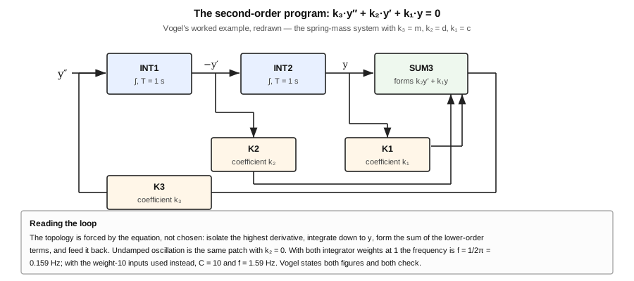
Figure 1 — The second-order program, redrawn from the workbook’s own block diagram. This one patch, with k₂ set to zero or not, produces the spring-mass system, the damped oscillation and the undamped oscillator — three of the workbook’s twenty examples. Diagram authored for this dive.

6.1 About this Volume

The machine exists for its workbook. Vol 1 §2 argued that the complement of computing elements was chosen to fit a published set of problems rather than the other way round; this volume is that set of problems.

The workbook — Rechenbeispiele, eighteen pages, twenty examples in seven sections — is held in this project’s library in the original German and in translation. Every example in it consists of a circuit, a derivation and an oscillogram of the result. This volume works through all seven sections, re-deriving the arithmetic and checking the numbers. Where the arithmetic closes, this volume says so; where it needed care, it says that too.

Cross-references: Vol 2 for the patch field these programs occupy; Vol 3 and Vol 4 for the elements; Vol 5 §6 for the overload indicator that §2.2 below exists to justify.

---

6.2 Machine Units and Scaling

The workbook opens with its convention, and the whole of the machine’s arithmetic rests on it:

“In the following examples, the variables are specified in dimensionless machine units. The machine unit +1 corresponds to a calculation voltage of +10 volts, and the unit −1 corresponds to a voltage of −10 V.”

Three consequences of that sentence govern every program below.

All variables are dimensionless. A displacement, a velocity and an acceleration in the same program are all numbers between −1 and +1, and the physics lives entirely in the coefficients. This is what makes the same patch a spring-mass system, an RLC circuit or a population model.

The range is hard. Beyond ±1 the machine does not degrade gracefully; it saturates at the supply rails, at roughly ±14 V, and stops obeying the equation. Amplitude scaling — choosing the correspondence between the problem’s units and the machine’s — is therefore not an optional refinement. It is the first step of programming, and the workbook’s §1.2 exists to demonstrate what happens when it is got wrong.

Time scaling is barely available. Larger machines scale time by switching integrator capacitors or input resistors over decades. This machine offers exactly two integrator time constants, 1 s and 0.1 s, selected by which input socket a patch cord goes into. There is no time-scale control, and there is no repetitive operation (Vol 2 §8). A problem is run at one of two speeds, or it is not run.

Note — The workbook is explicit that it is not a scaling textbook: “Programming details, such as variable and time normalization or the choice of initial conditions, are only discussed in these examples to the extent necessary for understanding.” Anyone approaching this machine with a problem of their own must do the scaling work elsewhere.

---

6.3 Section 1 — Basic Operations with Summers

6.3.1 Multiplication by a Constant

The workbook’s first example is the most instructive thing in it, because it shows that a summer with a transfer function of

y = −(x₁ + x₂ + 10·x₃)

is not one operation but a small family of them, depending only on where the patch cords go.

Table 1 — Multiplication by a Constant

Circuit	Patch	Result
a	one weight-1 input	y = −x
b	the same variable into two weight-1 inputs	y = −2x
c	one weight-1 input, output fed back to another weight-1 input	y = −0.5x
d	the weight-10 input, output fed back to both weight-1 inputs	y = −3.33x

Circuits c and d are the ones worth following, because they use the summer’s own feedback through the patch field rather than through the board.

For circuit c, the summer forms y = −(x + y). Rearranging: 2y = −x, so y = −0.5x. The element has become a coefficient potentiometer set to one half, without spending a potentiometer.

For circuit d, the input goes to the weight-10 socket and the output returns to two weight-1 sockets: y = −(10x + y + y). So 3y = −10x, and y = −3.33x.

Both derivations are the workbook’s own and both check. The technique they demonstrate — closing a loop from a summer’s output back into its own input to obtain a gain the hardware does not offer — is the single most useful trick on a machine with fixed feedback resistors, and it is worth the first page of the workbook.

Tip — Note what circuit d costs. A gain of −3.33 consumes all three inputs of one summer, leaving nothing for the sum it was presumably meant to form. On a machine with three summers, that is a third of the linear resource spent on one coefficient. A coefficient potentiometer would have done the same job for nothing; the point of the example is the technique, not the economy.

6.3.2 Sum of Three Variables, and the Example That Fails

The workbook’s §1.2 sets a target function

y = x₁ − 2.5·x₂ + 0.5·x₃ + 1

and patches it across three summers: S1 forms −(x₁ − 2.5·x₂ + 1), S2 forms −0.5·x₃, and S3 adds the two and inverts, giving y.

Numerical example 1 — x₁ = 0.4, x₂ = 0.2, x₃ = −1.0:

y = 0.4 − 2.5(0.2) + 0.5(−1.0) + 1
  = 0.4 − 0.5 − 0.5 + 1
  = 0.4                                  ✓ as the workbook states

Numerical example 2 — x₁ = −0.7, x₂ = 0.7, x₃ = 0.9:

y = −0.7 − 2.5(0.7) + 0.5(0.9) + 1
  = −0.7 − 1.75 + 0.45 + 1
  = −1.0

A result of exactly −1.0, which is on the boundary of the computing range but inside it. The machine nonetheless returns the wrong number, and the workbook says why:

y₁ = −(−2.5·x₂ + x₁ + 1)
   = −(−1.75 − 0.7 + 1)
   = **+1.45**

Summer S1 is asked to produce 1.45 machine units. It cannot. It saturates, and everything downstream of it is computing with a wrong input.

This is the most important example in the workbook, and it is worth stating why in general terms. The failure is invisible in three separate ways. The final answer is inside the range. Every input is inside the range. And the machine produces a stable, smooth, entirely plausible number. Nothing about the result announces that an intermediate value went out of range — which is precisely the class of error that the overload indicator described in Vol 5 §6 exists to catch, and precisely why that indicator monitors intermediate elements rather than only outputs.

The lesson the workbook draws is the operating discipline for the whole machine: scale so that every intermediate variable stays within ±1, not merely the answer. A program that satisfies the second condition and not the first is wrong and looks right.

6.3.3 A Linear System of Two Equations

The workbook’s §1.3 solves

x₁ + 0.5·x₂ − 0.3 = 0
0.2·x₁ + x₂ + 0.3 = 0

by rearranging each equation to isolate one unknown —

x₁ = −(0.5·x₂ − 0.3)
x₂ = −(0.2·x₁ + 0.3)

— and patching the two expressions directly, with each summer’s output feeding the other’s input. The workbook gives the solution as x₁ = 0.5, x₂ = −0.4, and both equations check:

0.5 + 0.5(−0.4) − 0.3 = 0.5 − 0.2 − 0.3 = 0     ✓
0.2(0.5) + (−0.4) + 0.3 = 0.1 − 0.4 + 0.3 = 0   ✓

This is an implicit program, and it is the one place in the workbook where the machine is used in a way that has no digital analogue at all. Nothing is integrated and nothing evolves; two amplifiers are cross-connected into an algebraic loop, and the loop has exactly one stable operating point — the solution of the system. The operator patches the equations and reads the answer off two elements. There is no algorithm, no iteration and no convergence criterion. The circuit is the solution, and it settles into it in microseconds.

Warning — An algebraic loop of this kind is stable only if the loop gain is below unity. Here the product of the two cross-coupling coefficients is 0.5 × 0.2 = 0.1, comfortably so. A system whose rearrangement produces a loop gain above one will latch at the rails instead of solving, and the machine gives no indication of the difference beyond the overload lamp. The workbook does not mention this condition.

---

6.4 Section 2 — Basic Operations with Integrators

6.4.1 Integrating a Constant

With one weight-1 input used, the integrator reduces to y = −∫x₁ dt − IC, and for a constant input a the elementary result is y = −a·t − IC: a straight line whose slope is the input and whose intercept is the initial condition.

The workbook’s demonstration is characteristic of the machine’s teaching style. A summer supplies the constant; the initial condition is set to +0.8; at t₀ the mode switch goes from IC to RUN and the output begins falling linearly. Part-way through, the key cable’s button is pressed, switching x₁ from +0.4 to −0.6. The output reverses direction — and the new line is steeper, because the magnitude of x₁ has also risen from 0.4 to 0.6.

Two properties of integration are made visible in one trace by one button press: that the input is the slope, and that the sign of the input is the direction. The oscillogram is recorded at 5 V per division and 1 s per division, which is to say the whole demonstration unfolds over several seconds and can be watched on the panel meter as well as a screen.

6.4.2 Integrating a Ramp

Adding a second integrator in series makes the input to the second a linear function of time, and its output therefore quadratic. The workbook’s oscillogram shows the pair started together at t₀, the first integrator’s input reversed at t₁, and — the detail it points out — an inflection in the second integrator’s output at every zero crossing of the first’s, which is the graphical statement of d²y/dt² = 0 where dy/dt changes sign.

Then, at t₂, both outputs run out of range:

“the outputs of the two integrators exceed their linear calculation range of ±10 V and run into the saturation range, which is determined by the level of the operating voltage (±15 V).”

This is the second demonstration of the same lesson as §1.2, in a dynamic setting: a program can start perfectly scaled and become unscaled as it runs. An integrator with a constant input will always reach saturation eventually; the only question is whether it does so before the interesting part of the solution is over.

---

6.5 Section 3 — Arithmetic with the Multiplier

Sections 3.1 to 3.4 — multiplication, division, squaring and square root — are covered in Vol 4 §3, where the device’s transfer equation and each patch are treated in full. The one example here that is a program rather than a demonstration of the element is §3.5.

6.5.1 Solving a Quadratic

The target is

y = x² − 0.7·x − 0.2

built from three elements: the first summer forms y₁ = −(0.7x + 0.2); the second forms y₂ = −(y₁ + x²), where x² comes from the multiplier in squaring mode; and an inverter gives y.

The workbook states the roots as x₁ = −0.22 and x₂ = +0.92. Checking by the quadratic formula:

x = [0.7 ± √(0.49 + 0.8)] / 2
  = [0.7 ± √1.29] / 2
  = [0.7 ± 1.1358] / 2
  = **+0.9179**  and  **−0.2179**

which rounds to the workbook’s figures. The arithmetic closes.

What the machine actually produces is not a pair of roots but a curve: the triangle generator sweeps x across the range, the program computes y for every value continuously, and the operator reads the roots off the zero crossings of an X–Y display. This is a different relationship with a quadratic than a digital solver offers — it shows the whole function and lets the roots be observed, rather than returning two numbers.

The workbook adds the expected caveat, and by now it is a familiar one: “for the range x ≤ −0.8 the calculation circuit is overloaded.” Sweeping the input across its full range drives an intermediate value out of the computing range at the negative extreme. The roots are nonetheless in the valid region, so the answer is good even though part of the displayed curve is not — a distinction an operator has to make consciously.

---

6.6 Section 4 — Trigonometric Functions

6.6.1 Sine

The direct case: x into terminal 39, sin x out of terminal 40, with the scaling x = φ/90° so that ±1 machine unit is ±90°. The workbook plots the transfer function and the time response to a triangular input, both at 2 ms per division — fast, because no integrator is involved.

6.6.2 Cosine

There is no cosine element. The workbook builds one from the identity

cos φ = sin(90° − φ)

which in machine units, where 1 corresponds to 90°, becomes

cos x = sin(1 − x)

A summer forms 1 − x from the reference and the variable, and the sine generator does the rest. But there is a complication the workbook handles carefully: cosine is an even function and the program must return positive values across the whole range −1 ≤ x ≤ +1, whereas sin(1 − x) would go negative for x < −1 + something. The workbook’s answer:

“To ensure this, the summing circuit is not supplied with the variable x, but with its absolute value |x|.”

So the cosine program is: absolute value (§5.3 below), then a summer forming 1 − |x|, then the sine generator. Three elements and a diode cable to obtain a cosine, on a machine that already has a sine. That is the honest cost of a fixed-function generator, and it is a good measure of what a variable DFG would have bought.

6.6.3 Double Angle

The workbook’s §4.3 is the most elaborate program in the book and uses more of the machine at once than anything else in it. It generates two harmonic variables from the integrator pair —

x₁ = cos x   and   x₂ = sin x

— using the quadrature oscillator of §7.2 below, multiplies them together, and applies the identity

sin 2x = 2·sin x·cos x

The multiplier’s product y* = x₁·x₂ is therefore ½·sin 2x: twice the frequency of its inputs but half the amplitude, which the workbook’s oscillogram shows plainly. A summer and an inverter then restore the factor of two, giving y = sin 2x.

The element count is worth tallying, because it shows the machine running near its limit: two integrators, one multiplier, one summer, one inverter, and the coefficient potentiometers to set the oscillator. That is every amplifier in the machine except two summers. This program could not be extended to sin 3x without running out of hardware.

Note also that this program does not use the sine generator at all. The sine and cosine come from the integrator loop, not from the diode ladder — because the quadrature oscillator produces both simultaneously and in phase quadrature, which is exactly what the identity needs and which a single-function generator cannot supply.

---

6.7 Section 5 — Discontinuous Functions

All three programs in this section use the open amplifier of Vol 3 §5 together with the diode cable of Vol 2 §6. Neither the amplifier nor the cable is a comparator; together they are.

6.7.1 Comparison of Two Variables

x₁ goes to one input of the open amplifier, and the inverted x₂ to another. With no feedback element, the amplifier’s gain resolves any difference into a saturated output:

x₃ = −U_S   for x₁ > x₂
x₃ = +U_S   for x₁ < x₂

where the saturation voltages are given as approximately ±14 V — outside the machine’s ±10 V computing range, which is the point. The raw comparator output is not a machine variable and must be conditioned. The workbook’s chain:

1. A diode suppresses the positive excursions, leaving only the negative half.

2. A coefficient potentiometer limits the survivor to −1, converting an uncontrolled −14 V into exactly one negative machine unit.

3. An inverter flips it, giving

   y = +1  for x₁ > x₂
   y =  0  for x₁ < x₂

A clean logic level, from an analog amplifier and two passive parts in a cable. The oscillogram is recorded at 2 ms per division with a triangular x₁ against a constant x₂, so the transitions can be seen sharply.

6.7.2 The Signum Function

Setting x₂ = 0 in the comparator program yields y = sign x directly, and the workbook notes the economy: “Because x₂ = 0 the inverter is of course no longer required here.” One element saved by recognising that a comparison against zero needs no reference input.

6.7.3 Absolute Value

The most elegant of the three, and the one that uses the open amplifier’s summing-point terminal properly.

Two diodes — the diode cable, with its midpoint contact — are arranged around the open amplifier so that the amplifier’s behaviour depends on the sign of its input:

• For positive x, D1 is blocked and D2 conducts, closing the feedback path. The amplifier is a plain inverter: x* = −x.
• For negative x, D2 is blocked. The feedback path opens, and the output is held at x* = 0.

A following summer then forms

y = −(x + 2·x*)

and the two cases resolve:

x > 0:   y = −(x + 2(−x)) = −(x − 2x) = **+x**
x < 0:   y = −(x + 0)     = **−x**

so y = |x| across the range. The arithmetic closes in both branches.

The trick worth noticing is the weight of two on x*. The program does not switch anything; it adds a correction that is zero for one sign of the input and exactly twice the right amount for the other. That is the characteristic shape of analog discontinuous programming — a continuous sum whose terms switch themselves on and off.

---

6.8 Section 6 — First-Order Differential Equations

6.8.1 y′ = y

The patch is two elements: assume y′ is present at the integrator’s input, so −y appears at its output; feed that output back to the input through an inverter, and the equation is satisfied. The solution is the exponential

y(t) = y(0)·e^t

with the integrator’s time constant T = 1 s setting the rate. The workbook records three runs at different initial conditions, captured one after another and superimposed afterwards — a direct consequence of the machine’s lack of repetitive operation, and a good illustration of how that absence shapes the way results are presented.

This program is also, as Vol 4 §6 notes, the machine’s only route to an exponential function. There is no exponential element; there is a differential equation whose solution happens to be one.

6.8.2 y′ = −k·y

The same patch with the inverter replaced by a coefficient potentiometer, since −k·y rather than y must return to the input:

y(t) = y(0)·e^(−k·t)

The workbook plots families of solutions for several k. This is where a demonstration machine earns its keep against a plot on paper: the operator turns one knob and watches a decay rate change continuously, which is a different kind of understanding from reading three curves.

---

6.9 Section 7 — Second-Order Differential Equations

6.9.1 The General Case

Given

k₃·y″ + k₂·y′ + k₁·y = 0

the highest derivative is isolated:

y″ = −(1/k₃)·(k₂·y′ + k₁·y)

and the patch follows mechanically, as Figure 1 of this volume shows. Assume y″ at the first integrator’s input; its output is −y′; the second integrator’s output is y; a summer forms −(k₂y′ + k₁y); and coefficient potentiometer k₃ returns that sum to the first integrator’s input. Two integrators, one summer, three potentiometers, and the two initial conditions set on the integrators.

The workbook then makes the equation physical. In mechanics this is a spring-mass system defined by mass m, spring constant c and damping constant d:

m·y″ + d·y′ + c·y = 0

so that k₃ = m, k₂ = d, k₁ = c — and the workbook flags the one thing that changes about the arithmetic: “In contrast to all previous calculation examples, the coefficients k₁ to k₃ here are not dimensionless.”

Its oscillograms then vary one coefficient at a time, all recorded at 1 s per division:

Table 2 — Its oscillograms then vary one coefficient at a time, all recorded at 1 s per division

Figures	Held constant	Varied	Shows
7.1, 7.2	k₃ = 0.8, k₂ = 0.01, y(0) = −1, y′(0) = 0	k₁ = 0.2 and 0.8	the effect of spring force on frequency
7.3 – 7.6	k₃ = 0.8, k₁ = 0.8, y(0) = −1, y′(0) = 0	k₂ = 0.02, 0.2, 0.5, 1.0	the progression from barely damped to heavily damped

That second set is the machine at its best. Four traces, one knob, and the whole qualitative story of damping — oscillatory, decaying, critical, overdamped — obtained by turning k₂ from 0.02 to 1.0 and photographing the screen four times.

6.9.2 The Undamped Oscillator

Setting k₂ = 0 removes the damping term and leaves

y″ = −(k₁/k₃)·y = −ω²·y

The workbook derives the frequency from the integrator weights. With both integrators at time constant T = 1 s and weight factor C, the first integration gives y′ = C·ω·cos ωt and the second y = C²·sin ωt; matching against y″ = −ω²·sin ωt requires ω = C, and since ω = 2πf,

f = C / 2π

For C = 1 — both loops through weight-1 inputs — that is f = 0.159 Hz, a period of about six seconds. For C = 10 — the weight-10 inputs — it is f = 1.59 Hz. Both figures are stated in the workbook and both check against f = C/2π.

The workbook’s closing observation on this program is the most honest sentence in it:

“Since in practice there is no arithmetic amplifier with ideal properties and no integration capacitors without losses, a weak oscillation damping occurs in the arithmetic circuit. As a result, the amplitudes of the two sine signals decrease slowly.”

A mathematically undamped oscillator, built from real parts, decays. The machine shows its own imperfection in the result, and the workbook prints it rather than cropping the oscillogram at two cycles.

Note — The companion workbook for the valve machine (Vol 7 §3) gives the same derivation with different numbers: C = 2 for both integrator inputs paralleled, giving f = 0.318 Hz. The two are not in conflict — they describe different machines with different input weight sets. A reader consulting both should not try to reconcile the figures.

---

6.10 What the Element Census Does to Programming

Collecting the demands the twenty examples make:

Table 3 — Collecting the demands the twenty examples make

Program	Integrators	Summers	Open amp	Pots	Multiplier	Sine
Sum of three variables (§1.2)	—	3	—	3	—	—
Linear system (§1.3)	—	2	—	3	—	—
Ramp integration (§2.2)	2	1	—	1	—	—
Square root with conditioning (Vol 4 §3.4)	—	1	1	2	1	—
Quadratic (§3.5)	—	2	1	2	1	—
Cosine (§4.2)	—	1	1	1	—	1
Double angle (§4.3)	2	1	1	2	1	—
Absolute value (§5.3)	—	1	1	—	—	—
Second order (§7.1)	2	1	—	3	—	—
Machine holds	2	3	1	4	1	1

No program exceeds the machine, and the double-angle program comes within one summer of exhausting it. That is not a coincidence — it is Vol 1 §2’s claim demonstrated: the complement was chosen to fit this list.

Three programming constraints follow from the table, and they are what an operator arriving with a new problem will meet first.

Sign management is the scarcest resource. Every summer, integrator and open amplifier inverts. A program’s signs must be made to work out by choosing where inversions fall, and when they cannot be, an element must be spent on an inverter. There is exactly one element — the open amplifier — that can be an inverter without also being something else, and the discontinuous programs of §5 need it.

Two integrators is the ceiling. Nothing above second order can be solved on this machine. A third-order system, a coupled pair of second-order systems, or any problem requiring a spare integrator for a stimulus ramp, is out of reach.

Every intermediate variable must be scaled, not just the answer. §1.2 and §2.2 and §3.5 all demonstrate the same failure from different directions. The overload indicator watches one element at a time (Vol 5 §6), so the discipline is: patch the program, then walk the address selector across every element in it while the problem runs, and only then believe the result.

---

6.11 What Comes Next

Vol 7 turns to the valve sibling of 2010 — a machine with the same programming philosophy, a different technology and a companion workbook that repeats much of this one at ±50 V — and then to the two documented replications and the part substitutions they made. It closes with a consolidated bench reference drawing on all six preceding volumes.