Vogel homebrew analog computer — Volume 5 — Reference, supply, metering and monitoring

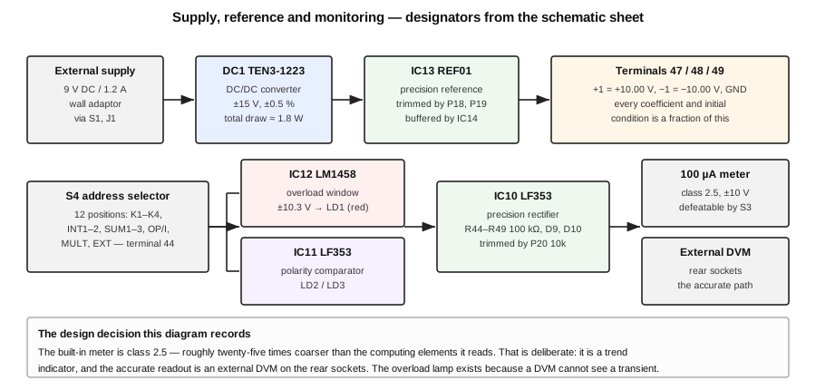
Figure 1 — The non-computing half of the machine, with designators from the schematic sheet. Diagram authored for this dive.

5.1 About this Volume

Six of the machine’s twelve integrated circuits do no computing at all. This volume covers all six, together with the converter and the reference they depend on: IC13 and IC14 (reference), IC10 and IC11 (rectifier, buffer and polarity), IC12 (overload), IC9 (triangle generator) and DC1 (supply).

This is not an appendix to the computing volumes. As Vol 1 §9 argues, the division of the board between computing and everything-else is the honest lesson of the design: the arithmetic is cheap and the trustworthiness is expensive. This volume is the expensive half.

Cross-references: Vol 3 for the computing elements these circuits serve; Vol 3 §6 for why the address selector’s coefficient-potentiometer positions exist; Vol 2 §7 for the panel controls that reach these circuits; Vol 6 for what an operator actually does with them.

---

5.2 The Reference Chain

Every coefficient the operator sets, every initial condition, and every constant term in every program on this machine is a fraction of one voltage. The reference is therefore not a supply — it is the machine’s definition of the number one, and its stability is the ceiling on everything else.

Table 1 — The Reference Chain

Designator	Value / type	Role
IC13	REF01	precision voltage reference; V/IN on pin 2, VOUT on pin 6, TRIM on pin 5, GND on pin 4
C21	0.1 µF	reference input decoupling
R41	470 kΩ	to the TRIM pin
P18	10 kΩ	trims the positive reference
R42	100 kΩ	inverter input
P19	2 kΩ	trims the inverter gain
R43	100 kΩ	inverter feedback
IC14	LF353	buffer and inverter
—	—	terminal 47 = +1; terminal 48 = −1; terminal 49 = ground

The architecture is worth reading carefully, because it explains why there are two trimmers rather than one.

The positive reference is generated; the negative reference is manufactured from it. IC13 produces the positive value, adjusted to exactly +10.00 V by P18 acting through R41 on the device’s own trim pin. That voltage then passes to an inverting stage built from R42 and R43 — nominally equal at 100 kΩ, and therefore nominally unity gain — around IC14, producing −10.00 V. P19, at 2 kΩ in that path, trims the inverter’s gain so that the negative reference matches the positive.

Two consequences follow, and both are properties of the machine an operator should know.

The two references are not independent. A drift in IC13 moves both. That is the right architecture for an analog computer, because what matters is not the absolute value of the reference but the symmetry of ±1 — a program that forms x − y from a positive and a negative reference sees only the difference between them. A pair of independent references would have twice the ways to go wrong.

Calibration has an order. P18 must be set before P19, because P19 adjusts a ratio against a quantity P18 defines. Setting them in the other order requires setting both twice. The sources do not state this; it follows from the topology.

Note — The description says only that the two references “can be calibrated to +10.00 V and −10.00 V” with “adjustment controls”. It does not name them, give their order, or say against what. A 4½-digit voltmeter at the panel’s +1 and −1 terminals is the obvious answer and is what the coefficient-setting procedure in Vol 3 §6 assumes, but the procedure is reconstructed here rather than quoted.

5.2.1 What the Reference Has to Drive

The four coefficient potentiometers are 10 kΩ each. A potentiometer patched across the reference draws 10 V ÷ 10 kΩ = 1 mA, and a program using all four draws 4 mA from the reference chain, plus whatever the computing elements take from the reference terminals directly.

That is not a trivial load for a reference, and it is the most likely reason the negative side is buffered by a dedicated amplifier rather than taken from a resistive divider. It is also a reason to prefer coefficient potentiometers of higher resistance in any reconstruction — a point Vol 7 §4 returns to, since one documented replication used pots as integrator input resistors and thereby changed the loading picture entirely.

Note — The 1 mA per potentiometer figure is arithmetic performed here. No held source discusses the reference chain’s load.

---

5.3 The Supply

Table 2 — The Supply

Designator	Value / type	Role
J1, S1	—	9 V DC input socket and power switch
DC1	TEN 3-1223	DC/DC converter: +9 V on pins 22/23, 0 V on pins 2/3; +15 V on pin 14, ground on pins 9/16, −15 V on pin 11
C19, C20	0.1 µF	output decoupling, one per rail

The whole of the machine’s power system is one module and two capacitors. The external adaptor is specified as 9 V DC at 1200 mA; the converter produces ±15 V stabilised to ±0.5 %; total machine consumption is given as approximately 1.8 W.

The module photographed on a board built to this design carries the marking TEN 3-1223 / IN 9-18VDC / OUT ±15VDC/±100mA, which agrees with the schematic’s designator and fills in two figures the sheet does not give: a wide input range and a per-rail current capability.

That last figure permits a useful check.

1.8 W at 9 V in          ≈ 200 mA from the adaptor
at a converter efficiency of roughly 75–80 %
                         ≈ 1.4 W delivered to the ±15 V rails
                         ≈ 47 mA per rail

Against a module rated at ±100 mA, the machine runs at roughly half the converter’s capability — comfortable, and consistent with twelve small-signal integrated circuits, three indicator LEDs and up to 4 mA of potentiometer load. The published 1.8 W is a credible figure rather than a round one.

Note — The efficiency assumption above is the analyst’s, not the manufacturer’s; no converter datasheet is held here. The check establishes that the stated consumption is of the right order, not that it is exact.

5.3.1 The Consequence Nobody Writes Down

A DC/DC converter is a switching supply, and this one sits on the same 105 × 88 mm board as six computing amplifiers whose summing junctions are being asked to resolve microvolts. That is the hardest electrical problem in the machine, and the schematic’s answer to it is visible in the component count: twelve 0.1 µF decoupling capacitors on the computing amplifiers alone, one per rail per device, with two more on the multiplier and further pairs through the auxiliary circuits.

There is no bulk reservoir drawn anywhere on the computing side and no filter between the converter and the rails beyond C19 and C20. The design relies entirely on local decoupling. A builder who economises on those capacitors — a reasonable-looking economy, since they are the most numerous part in the machine — will find switching residue on every output, and will find it worst on the integrators, which will integrate it.

Tip — One replication documented in Vol 7 §4 abandoned the DC/DC converter entirely in favour of a mains transformer with linear regulators, remarking only that a mains input was wanted. Whatever the motive, it removes this problem at a stroke, at the cost of the machine’s portability and its one-adaptor simplicity.

---

5.4 The Metering Path

Between any computing element’s output and the operator’s eye there are four circuit blocks, and each one is a decision.

5.4.1 The Address Selector

S4, a twelve-position rotary switch, brings the output of any computing element or coefficient potentiometer to a single node — terminal 44 — with no patching. Its positions, as drawn:

Table 3 — S4, a twelve-position rotary switch, brings the output of any computing element or coefficient potentiometer to a single node — terminal 44 — with no patching. Its positions, as drawn

Positions	Selects
1–4	K1, K2, K3, K4 — the coefficient potentiometers
5–6	INT1, INT2
7–9	SUM1, SUM2, SUM3
10	OP/I
11	MULT
12	EXT — an input socket on the programming field

Eleven of the twelve are hard-wired to element outputs; the twelfth is brought to the panel so that any node at all can be metered with one patch cord. From terminal 44 the signal goes two ways at once: to a switch offering the external DVM sockets on the rear of the case, and into the machine’s own metering chain through a buffer — IC11 with R55 at 3.3 MΩ, a deliberately high value that keeps the metering chain from loading the element being read.

Four of the twelve positions monitor coefficient potentiometers, which compute nothing and produce no answers. Vol 3 §6 explains why they are there: a 10 kΩ potentiometer driving a 100 kΩ summer input delivers up to 2.4 % less than its dial says, and the only way to set a coefficient correctly is to read the voltage it actually delivers, in circuit, through this switch.

5.4.2 The Precision Rectifier

Table 4 — The Precision Rectifier

Designator	Value	Role
IC10	LF353	both sections; precision rectifier
R44, R45, R46, R47, R49	100 kΩ each	the rectifier’s matched network
D9, D10	—	rectifying diodes inside the feedback loop
R48	91 kΩ	meter series resistor
P20	10 kΩ	meter calibration
S3	—	disables the panel meter
—	—	movement: 100 µA

A precision rectifier is a full-wave rectifier with its diodes inside an amplifier’s feedback loop, so that the amplifier’s gain divides out the diodes’ forward drop and the circuit rectifies accurately down to millivolts. It is a well-understood building block and this is a textbook implementation of it, with five matched 100 kΩ resistors and two diodes.

The question it raises is the interesting part of this volume. Why does a meter of accuracy class 2.5 need a precision rectifier? The movement is a ±2.5 % instrument reading a machine whose computing elements are good to 0.1 %. Rectifying its drive signal to a fraction of a percent buys nothing that the movement can display.

The economical answer is that the rectifier is not there for accuracy. It is there because the movement is a 100 µA single-polarity instrument being used to display a bipolar variable. Without rectification, a negative variable would drive the needle backwards against its stop. With it, the needle shows magnitude — and the sign is displayed separately, by the polarity lamps in §5 below. The precision part is then simply what falls out of doing the rectification with an op-amp rather than a diode, which costs one more device and removes the forward-drop error that would otherwise make small readings meaningless.

Note — That reading is inference. The sources describe the rectifier’s existence only through the schematic and describe the meter as having “a display range of ±10 V” with an LED polarity indicator. No source explains the choice.

5.4.3 The Meter Itself, and the DVM

The description is unusually candid about the panel meter:

“It has an accuracy class of 2.5 and is therefore far below the accuracy of the computing components. However, it is very suitable for purely qualitative demonstrations or for the trend display of a variable.”

And then, immediately:

“For precise static measurements, the analog computer features a parallel output for an external digital voltmeter, which can be connected via sockets on the rear of the case.”

This is the machine’s readout philosophy stated plainly, and it is the right one for a demonstration computer. The needle is for watching; the DVM is for measuring. A needle climbing steadily across a scale shows an integration happening in a way no digital display can, which is the entire point of a machine built to demonstrate. When a number is wanted, a four-digit instrument is plugged into the back.

Switch 6 on the panel — S3 on the sheet — disconnects the movement, so that a DVM or an oscilloscope sees the node without the metering chain across it.

---

5.5 The Polarity Indicator

Table 5 — The Polarity Indicator

Designator	Value	Role
IC11	LF353	comparator section (the package’s other section is the selector buffer)
R50	100 kΩ	input
R51	470 kΩ	positive feedback — hysteresis
R52	2.2 kΩ	—
R53, R54	5.6 kΩ	LED series resistors
LD2	—	POS, terminal 42
LD3	—	NEG, terminal 43

Two lamps, driven from the selected variable’s sign, restoring the information the precision rectifier removed. The presence of R51 at 470 kΩ as positive feedback around the comparator is the detail worth noting: it gives the stage hysteresis, so that a variable sitting near zero produces a clean indication rather than both lamps flickering. On a machine whose interesting moments are frequently zero crossings — every oscillatory program passes through zero twice a cycle — that is not a refinement.

Tip — One documented replication replaced the two lamps with a single bi-colour red/green LED, to save a hole in the front panel. The circuit supports it directly, since the two drives are complementary. See Vol 7 §4.

---

5.6 The Overload Indicator

Table 6 — The Overload Indicator

Designator	Value	Role
IC12	LM1458	dual comparator — the machine’s only non-BiFET amplifier
R35	4.7 kΩ	from +15 V
R36	10 kΩ	upper threshold leg
R37	10 kΩ	lower threshold leg
R38	4.7 kΩ	to −15 V
D11, D12	—	output steering
R39	5.6 kΩ	LED series resistor
LD1	—	OVL, terminal 46

The description states the function and the numbers:

“The switching thresholds of the monitoring circuit are set to ±10.3 V or ±1.03 machine units. If the monitored variable exceeds these limits, the overload condition is signalled by a red LED.”

That claim can be checked against the divider as drawn, and it is worth checking because it is the one place in the machine where a stated performance figure is fully determined by four resistor values.

Total chain  R35 + R36 + R37 + R38 = 4.7 + 10 + 10 + 4.7  = 29.4 kΩ
Across +15 V to −15 V                                     = 30 V
Chain current           30 V ÷ 29.4 kΩ                    = 1.0204 mA
Drop across R35         1.0204 mA × 4.7 kΩ                = 4.796 V
Upper threshold         +15 V − 4.796 V                   = **+10.20 V**
Lower threshold         −15 V + 4.796 V                   = **−10.20 V**

Against a published ±10.3 V, that is agreement to within 1 % — comfortably inside the tolerance of the resistors and the offsets of an LM1458. The machine’s stated overload threshold is exactly what its own parts produce.

Note — The arithmetic above is analysis performed for this series. Its interest is not the third digit but the confirmation: the description’s numbers are measured or computed from the real circuit, not rounded from intention. That is a useful thing to know about a source before trusting its other figures.

5.6.1 Why the Lamp Exists at All

The description gives the reason in one sentence, and it is the best single justification for a monitoring circuit anywhere in this hub’s machines:

“Temporary overloads of computing elements cannot be detected with a digital voltmeter.”

An analog computer’s characteristic failure is silent. An amplifier driven past its linear range stops obeying the equation, and thereafter produces a smooth, plausible, entirely wrong curve. If the excursion happens for fifty milliseconds in the middle of a five-second run, a DVM reading the output at the end shows a perfectly sensible number, and there is nothing in the answer to indicate that the machine stopped solving the problem part-way through.

The workbook makes this concrete rather than theoretical. Example 1.2 is a three-variable sum whose result, y = −1.0, lies safely inside the computing range — and which the machine nonetheless gets wrong, because an intermediate result inside the program reaches 1.45. Vol 6 §2 works that example through. The lamp is the machine’s answer to that class of error, and it watches whichever element the address selector has selected.

Warning — The overload indicator monitors one element at a time — whichever the address selector has chosen. It is not a machine-wide alarm, and a program can be overloading an element the operator is not currently watching. The discipline the machine implies is to walk the selector across every element in a program before trusting any answer from it.

---

5.7 The Triangle Generator

Table 7 — The Triangle Generator

Designator	Value	Role
IC9	LF353	both sections: integrator and comparator
C22	33 nF	timing capacitor
R56	100 kΩ	—
R57, R58	180 kΩ each	comparator threshold network
D13, D14	—	with P31 and P32
P31, P32	5 kΩ each	slope symmetry adjustment
P33	10 kΩ	frequency — the multi-turn control on the side of the case
R59	220 Ω	—
—	—	output on terminal 45, panel group K

The circuit is the classic relaxation oscillator: an integrator and a comparator in a loop, the comparator’s square output driving the integrator, the integrator’s triangle output switching the comparator. The description gives the specification as ±10 V output, 1.5 Hz to 75 Hz.

The reason it is in the machine is stated precisely: it is “for specifying defined, linearly time-dependent variables”. That is, it is not a test oscillator. It is the machine’s source of the variable t.

Nothing else in the complement produces a controlled ramp. An integrator fed a constant will produce one, but doing so spends an integrator — of which there are two — on a job that contributes nothing to the equation being solved. For every program in the workbook that plots a function rather than solving a differential equation, the triangle generator supplies the independent variable and the element under study supplies the dependent one, and the pair is displayed on an oscilloscope in X–Y. That is how the workbook’s transfer-function plots of the multiplier and the sine generator were made, and it is why those oscillograms are recorded at 2 ms per division while the differential-equation solutions are recorded at 1 s per division.

Two adjustments, P31 and P32, work with D13 and D14 on the two halves of the waveform separately — a rising-slope trim and a falling-slope trim. Their purpose is to make the two ramps symmetric so that the waveform is a true triangle. The frequency control P33 is the only preset in the machine brought out to the operator, and it is on the side of the case rather than the face, which places it correctly: it is a setting made once per experiment, not part of a program.

---

5.8 The Adjustments, and What Is Not Documented

Collecting every potentiometer on the sheet:

Table 8 — Collecting every potentiometer on the sheet

Designator	Value	Purpose	Documented?
P1 – P6	50 kΩ	offset null, one per computing amplifier IC1–IC6	implied by the topology; no procedure given
P11	50 kΩ	sine generator input level	no
P12	1 MΩ	sine generator, innermost segment slope	no
P13 – P17	500 kΩ	sine generator, outer segment slopes	no
P18	10 kΩ	positive reference trim	yes — “adjustment controls”
P19	2 kΩ	negative reference trim	yes — as above
P20	10 kΩ	meter calibration	no
P21 – P24	10 kΩ	the four coefficient potentiometers (panel)	yes
P31, P32	5 kΩ	triangle generator slope symmetry	no
P33	10 kΩ	triangle generator frequency (side of case)	yes

That is eighteen internal preset adjustments, one side-mounted operator control, and four panel potentiometers. Of the eighteen presets, the held sources explain two.

No calibration or alignment procedure for this machine exists in the held record. There is no order of operations, no statement of what each trimmer is set against, and no acceptance criterion. What can be reconstructed from the circuits is the following, and it is offered as reconstruction:

1. P18, then P19 — reference first, since everything else is measured against it, and in that order for the reason given in §2.
2. P1 to P6 — amplifier offsets, each nulled with its element’s inputs grounded and its output watched on a DVM. These are the six that most reward doing, because an integrator’s offset integrates.
3. P20 — meter calibration, against the reference on a known selector position, once the reference is right.
4. P31, P32 — triangle symmetry, on an oscilloscope, independent of everything else.
5. P11 to P17 — the sine generator last and by a long way, because seven interacting adjustments shaping a piecewise-linear curve is a different order of task. Vol 4 §3 sets out what is involved.

Note — The numbering itself is worth recording, because it is informative and because its gaps might otherwise look like missing components. The sheet uses P1–P6, P11–P24 and P31–P33; P7–P10 and P25–P30 do not appear. The pattern is a reserved-block scheme — ten numbers for amplifier offsets, ten for the analog function blocks, ten for panel potentiometers, and a further block for the generator — of which the machine uses part of each. Nothing is missing.

---

5.9 What Comes Next

Vol 6 turns to programming: machine units, scaling, and the twenty published worked examples re-derived and checked — including the one in §2 that returns a confidently wrong answer, which is the reason the overload lamp described above is in the machine. Vol 7 covers the valve sibling, the two documented replications and their substitutions, and closes with a consolidated bench reference drawing on all six preceding volumes.