Vogel homebrew analog computer — Volume 4 — The non-linear elements

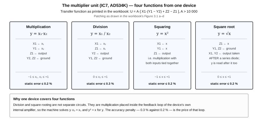
Figure 1 — The multiplier unit’s four functions. Terminal assignments are as drawn in Figure 3.1 a–d of the workbook; equations and error figures as printed in the workbook and the 2009 description. Diagram authored for this dive.

4.1 About this Volume

The machine contains exactly two non-linear computing elements: a four-quadrant multiplier unit built around one integrated circuit, and a diode function generator that approximates a sine by eleven straight lines. Between them they carry every operation in the machine that a summer and an integrator cannot perform.

This volume walks both with the schematic sheet open, and works the multiplier’s four functions through algebraically from the device’s transfer equation. As in Vol 3, transcribed material and analysis are distinguished in the sentence that presents them.

Cross-references: Vol 2 §4 for the MUL and SIN columns on the panel; Vol 3 for the linear elements these two work alongside; Vol 5 §7 for the triangle generator that drives every transfer-function plot in this volume; Vol 6 §3 and §4 for the programs.

---

4.2 Why These Two Elements Carry So Much

A summer and an integrator are both linear: whatever they do to a sum of inputs, they do to each input separately and add the results. Every problem expressible with them alone is a linear one, and linear problems are a small and rather dull corner of the space an analog computer exists to explore.

Everything interesting is non-linear, and on this machine everything non-linear passes through one of these two elements or through the open amplifier’s saturation. That makes the complement worth stating explicitly, because the boundary is sharper than on a larger machine:

Table 1 — Everything interesting is non-linear, and on this machine everything non-linear passes through one of these two elements or through the open amplifier's saturation. That makes the complement worth stating explicitly, because the boundary is sharper than on a larger machine

Operation	Element	Where
x₁ · x₂	multiplier	§3.1
x₁ / x₂	multiplier	§3.2
x²	multiplier	§3.3
√x	multiplier	§3.4
sin x	sine generator	§4
cos x	sine generator + summer + absolute value	Vol 6 §4.2
sin 2x	two integrators + multiplier + summer	Vol 6 §4.3
sign x, |x|, comparison	open amplifier + diode cable	Vol 6 §5
arbitrary f(x)	none — the machine cannot do this	—
log, exp	none	—

The last two rows matter. A larger analog computer of the period offered a variable diode function generator: a row of ten or twenty potentiometers setting the slope of successive segments, letting the operator dial in any single-valued function by hand. The EAI TR-10 offered three models of exactly that. This machine has no such element. Its diode function generator makes one function, sine, and its breakpoints are fixed by selected zener diodes soldered to the board. That is the sharpest expression of the design brief set out in Vol 1 §2: a demonstrator sized to a published problem set needs the functions those problems use, and no others.

---

4.3 The Multiplier Unit

4.3.1 The Device as Drawn

Table 2 — The Device as Drawn

Pin	Name	Connection on the sheet	Panel terminal
1	X1	to terminal 31	31
2	X2	grounded	—
4	SF	tied to the same point	—
6	Y1	to terminal 32	32
7	Y2	to terminal 33	33
8	−Vs	−15 V, decoupled by C16 (0.1 µF)	—
10	Z2	to terminal 34	34
11	Z1	to terminal 36	36
12	OUT	to terminal 35	35
14	+Vs	+15 V, decoupled by C15 (0.1 µF)	—

The device is lettered AD534K on the sheet. Five of its inputs reach the panel — X1, Y1, Y2, Z1, Z2 — and the description confirms the count: “By appropriately wiring its five inputs X, Y1, Y2, Z1, Z2, four calculation functions can be selected.”

Two pins are committed on the board and never reach the operator. X2 is grounded, which fixes the X input as single-ended rather than differential. SF — the scale-factor pin — is tied to the same point, which means the device’s denominator is whatever that connection produces and is not adjustable. The practical consequence for a programmer is that the multiplier’s scale factor is a property of the machine, not a parameter: the panel’s ±1 machine unit maps onto the device’s own full scale, and there is no way to change that from outside.

Note — No AD534 datasheet is held in this project’s library, so nothing about the device’s internal design, its scale-factor pin conventions or its temperature behaviour is asserted here beyond what the schematic shows and the two Vogel documents state. The description characterises the unit as working “according to the translinear principle”; that claim is reproduced, not checked.

4.3.2 The Transfer Equation

The workbook gives the device’s behaviour in one line, and every one of the four functions falls out of it:

U = A · [ X1·(Y1 − Y2) + Z2 − Z1 ], with A > 10 000

This is a differential multiplier followed by a very high-gain amplifier, with Z1 and Z2 as summing inputs to that amplifier. The high gain is the key to the whole arrangement: because A is enormous, any patch that closes a loop from OUT back into an input forces the bracket to zero, and the equation the bracket describes is then solved for the output. Two of the four functions are obtained that way.

Table 3 — The Transfer Equation

Bracket set to zero by feedback	Solved for y	Function
x₁·x₂ − y = 0	y = x₁·x₂	multiplication
−x₂·y + x₁ = 0	y = x₁ / x₂	division
x² − y = 0	y = x²	squaring
−y² + x = 0	y = √x	square root

4.3.3 Multiplication

Figure 3.1 a) of the workbook patches x₁ into X1, x₂ into Y1, the output back into Z1, with Y2 and Z2 grounded. Substituting into the transfer equation:

y = A·(x₁·x₂ − y)
y·(A + 1) = A·x₁·x₂
y = x₁·x₂            since A ≫ 1

Permitted range −1 ≤ x₁, x₂ ≤ +1; stated static error ≤ 0.2 %.

This is four-quadrant multiplication — both inputs may take either sign, and the product carries the correct sign — which is the property that makes the element worth having. A two-quadrant multiplier would be useless for the sin 2x program of Vol 6 §4.3, where both factors swing through zero twice per cycle.

4.3.4 Division

Figure 3.1 b) patches x₂ into X1 and x₁ into Z1, with the output taken back to Y2, and Y1 and Z2 grounded. The workbook’s substitution is:

y = A·(−x₂·y + x₁)
y·(1 + A·x₂) = A·x₁
y·x₂ = x₁           since A ≫ 1
y = x₁ / x₂

Permitted range −1 ≤ x₁ ≤ +1 and 0 ≤ x₂ ≤ +1; stated static error ≤ 0.3 %.

Three things about division deserve emphasis, because it is the mode most likely to misbehave in an operator’s hands.

The divisor is single-quadrant. x₂ must be positive. This is not a limitation of the device but of the loop: the feedback path’s polarity is fixed by the patch, and a divisor passing through zero and changing sign turns negative feedback into positive feedback. The machine will not warn about this; it will simply latch at a rail.

The accuracy is worse, and the reason is structural. 0.3 % against multiplication’s 0.2 % is the price of putting the multiplier inside a feedback loop rather than using it open. The loop’s residual error is divided by A, but the input error of the multiplying core is divided by x₂ — so the smaller the divisor, the larger the quotient and the larger the error on it.

The divisor cannot approach zero. As x₂ falls, the loop gain A·x₂ falls with it, and the approximation y·(1 + A·x₂) ≈ y·A·x₂ that produces the clean result stops holding. The workbook states the permitted range and does not discuss the degradation; the mechanism is visible in its own algebra.

Note — The reading of the three points above is analysis. The workbook states only the ranges and the error figures.

4.3.5 Squaring

Figure 3.1 c) is Figure 3.1 a) with x applied to X1 and Y1 together — one variable driving both factors, the output returned to Z1. Range −1 ≤ x ≤ +1; stated static error ≤ 0.2 %, the same as multiplication, which it is.

The workbook plots the resulting transfer function as its Figure 3.2 — a clean parabola from (−1, 1) through the origin to (+1, 1) — and its Figure 3.3 shows the time response to a triangular input, recorded at 5 V per division and 2 ms per division. That second oscillogram is worth a remark, because it shows how the machine is actually used to characterise an element rather than to solve a problem: the triangle generator sweeps x linearly, the multiplier produces x², and the two are displayed together. There is no integration anywhere in that measurement, which is why it can run at 2 ms per division on a machine whose only integrator time constants are 1 s and 0.1 s.

4.3.6 Square Root

Figure 3.1 d) is the subtlest patch in the machine. x goes to Z1. The output passes through a series diode, and it is the voltage after the diode that is taken back to both X1 and Y2 — and that is also where y is read. Y1 and Z2 are grounded. The workbook’s substitution:

y = A·(−y² + x) = A·x − A·y²
y² = x              since A ≫ 1
y = √x

Permitted range 0 ≤ x ≤ +1; stated static error ≤ 0.2 %.

The workbook explains the diode explicitly, and the explanation contains both of the things an operator needs to know:

“The diode inserted in the feedback circuit ensures that no negative voltages can occur at the inputs X1 and Y2. The result of the square root extraction circuit does not appear directly at the output of the multiplier unit, but only after the diode.”

The first clause is the loop’s stability condition. A square-root loop has two mathematical solutions, +√x and −√x, and it will happily find the negative one and stay there. The diode removes that half of the solution space by refusing to let the fed-back voltage go negative, so the loop can only settle on the positive root.

The second clause is the trap. Terminal 35 — the multiplier’s output socket — does not carry the answer in this mode. The answer is on the far side of the diode, which is a component in a patch cord, so the operator must read it at whatever node the diode’s output is patched into. An operator who patches square-rooting and then reads terminal 35 out of habit will get a voltage one diode drop above the true result, at every point on the curve.

4.3.7 Getting a Unipolar Input

Because square-rooting requires 0 ≤ x ≤ +1 and the machine’s only ramp source — the triangle generator — swings ±1, plotting a square-root transfer function needs a conversion stage in front of it. The workbook’s Figure 3.4 supplies one, and it is a small, clean piece of programming worth recording:

Table 4 — Because square-rooting requires 0 ≤ x ≤ +1 and the machine's only ramp source — the triangle generator — swings ±1, plotting a square-root transfer function needs a conversion stage in front of it. The workbook's Figure 3.4 supplies one, and it is a small, clean piece of programming worth recording

Element	Setting	Role
Coefficient potentiometer	k = 0.5	halves the ±1 triangle to ±0.5
Second coefficient potentiometer	k = 0.5	takes −1 reference to −0.5
Summer	weight-1 inputs	adds the two, giving 0 … +1
Inverter	—	restores the sign

Two potentiometers, a summer and an inverter — four of the machine’s scarce elements spent purely on conditioning a stimulus, before the problem itself has begun. On a machine with three summers and one open amplifier, that is a real cost, and it is a good illustration of why the workbook’s programs are as economical as they are.

---

4.4 The Sine Diode Function Generator

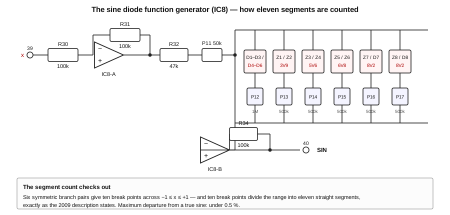
Figure 2 — The sine generator (IC8), redrawn from the schematic sheet. Diagram authored for this dive.

The description states what the element does and how well:

“The sine function is generated with a diode function generator by eleven straight lines. The break points are determined by selected Zener diodes. The diode function generator is for an input variable in range −1 ≤ x ≤ +1. The maximum deviation of the approximate curve from the mathematical course of the sine function is less than 0.5 %.“

4.4.1 Input Conditioning

Table 5 — Input Conditioning

Designator	Value	Role
—	—	terminal 39, the x input
R30	100 kΩ	input resistor
R31	100 kΩ	feedback — unity inverter around IC8 section A
R32	47 kΩ	series feed into the ladder
P11	50 kΩ	ladder drive level

The input passes through a unity inverter before it reaches the diode ladder. That inversion is not incidental: the ladder and the output amplifier each invert once more, and the three inversions together return the output to the same sign as the input, so that a positive x produces a positive sin x. P11 sets the amplitude of the signal presented to the breakpoint network, which is the master gain of the whole approximation — it scales every segment together, and is therefore the adjustment that sets the peak value of the generated sine.

4.4.2 The Breakpoint Ladder

Six branches, all symmetric about zero, each with a slope potentiometer beneath it:

Table 6 — Six branches, all symmetric about zero, each with a slope potentiometer beneath it

Branch	Devices	Breakpoint set by	Slope control
1	D1, D2, D3 in series / D4, D5, D6 in series	three silicon junctions, ≈ 1.8 V either way	P12, 1 MΩ, with R33 at 1 MΩ
2	Z1 / Z2	zener, 3V9	P13, 500 kΩ
3	Z3 / Z4	zener, 5V6	P14, 500 kΩ
4	Z5 / Z6	zener, 6V8	P15, 500 kΩ
5	Z7 / D7	zener, 8V2	P16, 500 kΩ
6	Z8 / D8	zener, 8V2	P17, 500 kΩ

The output is summed by IC8’s second section through R34 at 100 kΩ and appears at terminal 40.

4.4.3 Counting the Eleven Segments

The “eleven straight lines” of the description is checkable against the parts, and it checks.

Each branch conducts only above a threshold voltage, and above that threshold it adds a further current path into the summing node — which adds a further increment of slope. Six branches, each symmetric about zero, give six break points on the positive side and six on the negative. But the innermost branch, the silicon string, breaks at roughly ±1.8 V, which is not zero; the region between its two break points is the central segment.

central segment                                    1
positive side: 6 branch thresholds → 6 more        6
negative side: 6 branch thresholds → 6 more        6
                                                  ──
hmm — that gives 13, not 11

The count only comes right when one notices that the two outermost branches share a zener value: Z7 and Z8 are both 8V2, and Z5/Z6 at 6V8 sit just below them. With the ladder driven through P11 at a level that places the outermost pair at or beyond the ±1 extremes of the input range, the outermost break points fall outside the working range and never bend anything inside it — which reduces the count inside −1 ≤ x ≤ +1 to five effective break points per side, and

central segment + 5 per side × 2 sides = **11 segments**

exactly as stated.

Note — The reconciliation above is analysis, and it should be read as the most economical account rather than as a certainty. What is certain and transcribed is the parts list: six symmetric branches, with zener values 3V9, 5V6, 6V8, 8V2 and 8V2, plus a three-diode silicon string; and the description’s claim of eleven segments and better than 0.5 %. A reader with the machine can settle the mapping in an afternoon by sweeping the input and watching where the slope changes.

4.4.4 Why Zener Diodes Rather Than a Resistive Ladder

The conventional diode function generator of the period set its break points with a resistive divider chain from the reference supply: each diode’s cathode sat at a tapped voltage, and the diode began to conduct when the signal exceeded that tap. That is how larger machines did it, and it is how the valve sibling described in Vol 7 §2 does it — the 2010 document names R82 to R89 as the divider resistors that fix its break points.

This machine does it with zeners instead, and the trade is worth naming:

Table 7 — This machine does it with zeners instead, and the trade is worth naming

	Resistive divider	Selected zeners
Break points depend on	the reference supply	the diodes themselves
Parts count	one divider chain plus one diode per break	one zener per break
Adjustable	yes, by changing taps	no — resoldering only
Needs a reference feed	yes	no
Temperature behaviour	follows the reference	follows the zeners

For a machine whose function generator will only ever make one function, the zener scheme is plainly correct: it removes an entire divider chain and its connection to the reference, at the cost of an adjustability the design does not want. The word the description uses is “selected” zeners, which is the whole story — the break points are set by choosing parts at build time rather than by setting anything afterwards.

What remains adjustable is the slope of each segment, through P12 to P17. That is the right division: the break points are where the curve bends, and the slopes are how much. Getting the bends in the right places is a matter of buying the right diodes; getting the amounts right is seven interacting adjustments, which is why Vol 5 §8 places the sine generator last in any alignment.

4.4.5 Scaling the Sine

The element generates sin x for −1 ≤ x ≤ +1, which requires a convention relating the machine unit to an angle. The workbook states it:

“Using a scaling factor x = φ/90, the input variable x is thus proportional to an angle φ.”

So ±1 machine unit is ±90°, a quarter turn, and the generated curve is one full positive-and-negative lobe of a sine — from −1 through 0 to +1 as x sweeps −1 to +1. That is exactly the range a piecewise-linear approximation can cover with eleven segments at better than half a percent, and it is also the range over which sine is monotonic, which matters for any program using the element inside a loop.

Getting a cosine out of it requires the identity cos φ = sin(90° − φ), which in machine units is cos x = sin(1 − x) — a summer and the reference. But cosine is even and sine is odd, so the argument must be folded: the workbook’s cosine program feeds the summer |x| rather than x, using the absolute-value circuit of Vol 6 §5.3. Three elements and a special cable, to obtain a cosine from a sine generator. Vol 6 §4.2 works it through.

4.4.6 The Lettering Question

The sheet letters this device IC8 LM353. Every other dual amplifier on the same two pages — IC9, IC10, IC11 and IC14 — is lettered LF353, and the 2009 description characterises the machine’s amplifiers as BiFET throughout.

The most economical reading is a slip of the pen for LF353, and nothing about the circuit contradicts it: the stage is a unity inverter and a summing amplifier, which any general-purpose dual would perform. The reading is nonetheless inference, and this series does not adopt it silently. A builder working from the sheet should fit an LF353 and should know that they are correcting the drawing when they do.

---

4.5 What the Two Elements Cannot Do

Stated plainly, because a reader may come to this machine expecting otherwise:

• No arbitrary function generation. There is no variable DFG. A function other than sine cannot be dialled in; it can only be built out of the multiplier’s four operations and the elements in Vol 3.
• No logarithm or exponential. Neither element produces one, and neither does any combination of them. A program needing e^x uses an integrator in a feedback loop instead — which is exactly what the workbook’s §6.1 does, solving y′ = y and obtaining an exponential as the solution rather than as a function evaluation.
• No comparator. The multiplier and the sine generator are both continuous. Discontinuous behaviour comes from the open amplifier’s saturation and the diode cable, as Vol 3 §5 and Vol 6 §5 set out.
• No second multiplier. The sin 2x program of Vol 6 §4.3 needs one multiplier and gets it; a program needing two products simultaneously cannot be run.

---

4.6 What Comes Next

Vol 6 is the programming volume, and it puts every element described in Vols 3, 4 and 5 to work on the twenty published examples — including the multiplier’s four modes in operation, the sine, cosine and double-angle programs, and the three discontinuous functions. Vol 7 turns to the valve sibling, which has a diode function generator of the resistive-divider kind described in §4.4 above, and to the two documented replications, both of which had to substitute for the AD534K.