Homebrew & Open-Source Analog Computers — Volume 6 — Patching and scaling practice

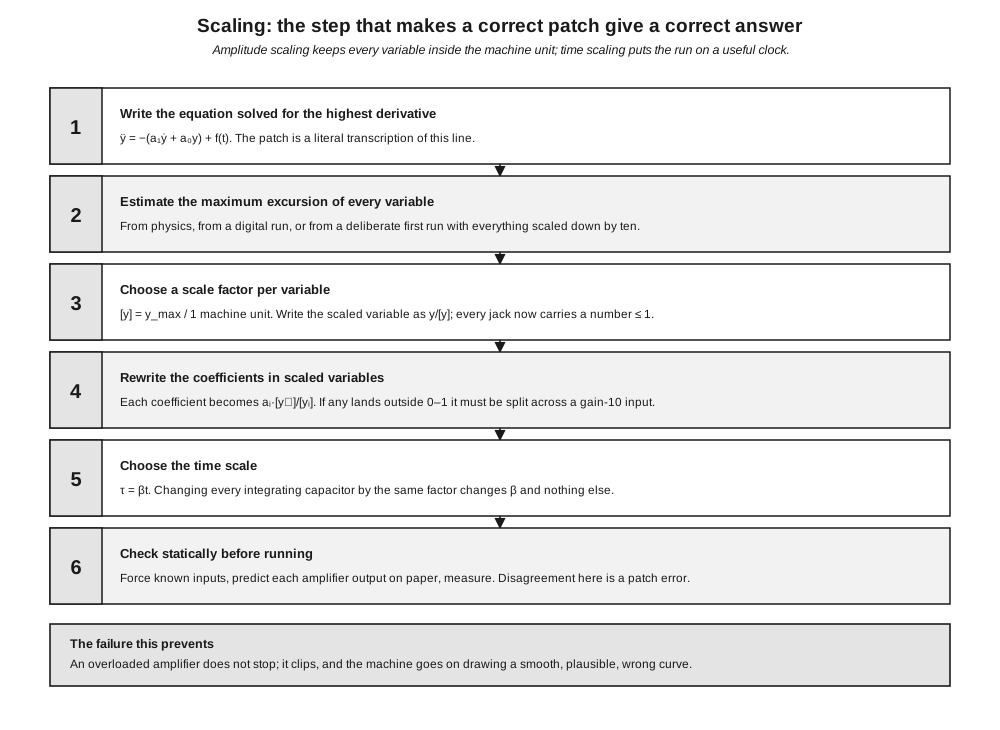
Figure 1 — The scaling procedure as a worksheet. Steps 1 to 4 are amplitude scaling, step 5 is time scaling, and step 6 is the discipline that makes the first five trustworthy. Diagram authored for this dive by build/make_diagrams.py.

---

6.1 About This Volume

A correctly built analog computer will solve the wrong problem without complaint. Vols 2 to 5 covered the hardware; this volume covers the part where most of the errors actually occur.

The work divides into three. Amplitude scaling keeps every variable inside the machine’s voltage range, because an amplifier driven past it clips and the equation it was implementing silently stops holding. Time scaling puts the solution on a clock that suits the readout. Check-out establishes that the patch on the machine is the patch that was intended, before any answer is believed.

Two programs are worked completely, with the arithmetic shown, because scaling is a procedure that is learned by doing it once properly rather than by reading a description of it.

Cross-references: Vol 2 for the element transfer functions; Vol 3 §6.1 for overload detection, which is the hardware half of §7; Vol 5 §6.4 for why the patch diagram is the only durable record of a program.

---

6.2 The Flow Diagram Is the Source Code

Before any voltage exists there is a drawing: the interconnection of computing elements that represents the equation, with every coefficient marked and every element numbered.

On a machine with no removable problem board — which is every design in Vol 1 §5 — this drawing is the only persistent form of the program. The patch cords are working storage and they are cleared the moment the next problem is set up. A builder who patches from memory and does not draw will have no way to re-run the work, no way to find an error systematically, and no way to hand the program to anyone else.

The drawing should carry four things: each element with its number as physically labelled on the machine, each coefficient with its computed value, the scale factor of every variable, and the initial condition of every integrator. Those four are exactly what §6 needs to verify the patch, and a diagram lacking them cannot be checked.

---

6.3 Amplitude Scaling

6.3.1 The Problem

The machine represents every variable by a voltage limited to one machine unit — ±10 V on most designs in this survey, ±100 V on the EEVblog machine of Vol 4 §7. The problem’s variables have their own units and their own magnitudes, and nothing guarantees they fit.

Scaling is the change of variable that makes them fit. For each problem variable $y$ a scale factor $[y]$ is chosen, and the machine computes the dimensionless $y’ = y/[y]$, which is held to a magnitude of one or less.

Two failures bracket the choice. Choose $[y]$ too small and the amplifier overloads, the equation stops holding, and the machine produces a smooth wrong curve. Choose $[y]$ too large and the variable occupies a small fraction of the range, so every fixed error — offset, noise, multiplier error — becomes a larger fraction of the signal. Good practice puts the expected maximum at something like 0.5 to 0.9 of full scale.

6.3.2 Estimating the Maxima

The scale factors depend on the maxima, which are what the machine is being asked to find. This apparent circularity is resolved in one of three ways, in descending order of rigour: analytically, where the system is linear and the bound can be derived; from physics, where the quantity has a known plausible range; or empirically, by running the problem once with everything deliberately scaled down by a factor of ten and observing what the variables actually do.

The third is entirely respectable and is what most operators do. It requires overload detection to be trusted, which is the argument of Vol 3 §6.1 restated from the programmer’s side.

6.3.3 Realising a Coefficient

Once scaled, every coefficient must be realised in hardware, and the hardware offers exactly two mechanisms (Vol 2 §3.1 and §5):

• a coefficient potentiometer, which supplies any factor from 0 to 1 and nothing above 1
• an input weight of 1 or 10, set by which input jack is used

Any coefficient up to 10 is therefore the product of a weight and a pot setting: a coefficient of 3.5 is the gain-10 input with the pot at 0.35. Coefficients above 10 require two elements in series, and a coefficient above 100 is a strong hint that the scaling is wrong and should be revisited rather than patched around.

The constraint that catches people is that a potentiometer cannot produce a negative coefficient. Negative coefficients must come from the sign of the signal being fed in, which is why the inverter count in a program is not a matter of taste. §4 shows this deciding a topology.

---

6.4 Worked Program: The Damped Oscillator

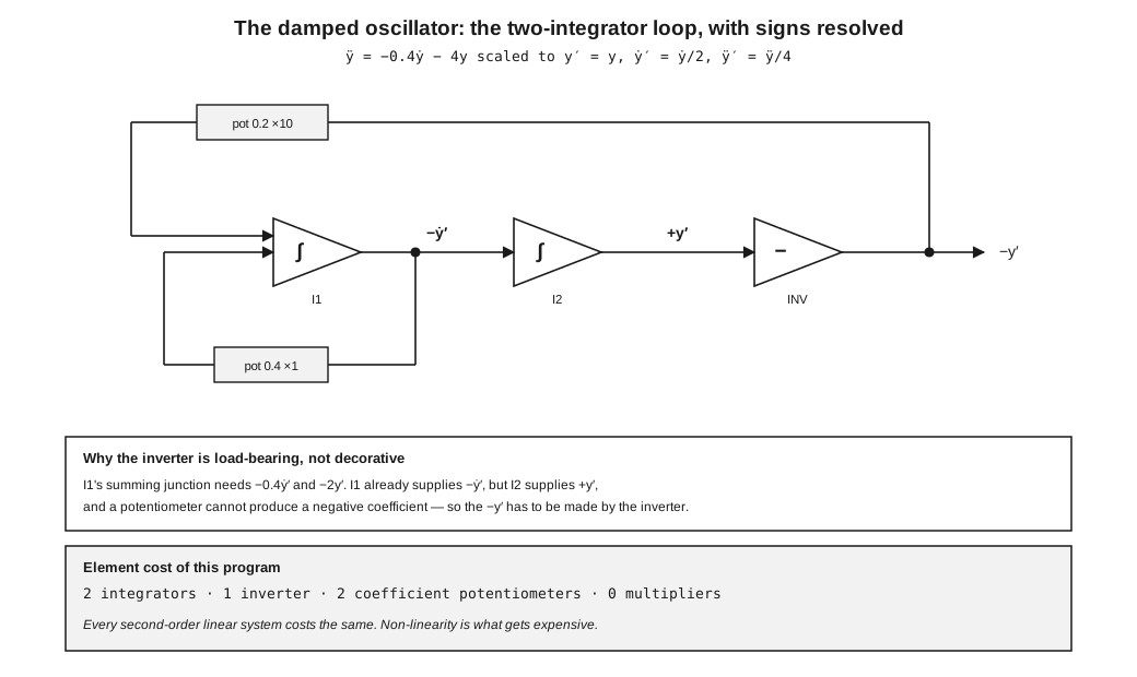
Figure 2 — The worked program of this section, with signs and coefficients resolved. The stiffness term is fed back from the inverter output rather than from the second integrator, for the reason set out in §4.4. Diagram authored for this dive by build/make_diagrams.py.

6.4.1 The Problem

A mass-spring-damper, written in the standard form and then solved for the highest derivative:

$$\ddot{y} + 2\zeta\omega_n\dot{y} + \omega_n^2 y = 0$$

Taking $\omega_n = 2$ rad/s and $\zeta = 0.1$:

$$\ddot{y} = -0.4,\dot{y} - 4,y$$

The machine is assumed to have integrators with $RC = 1$ s, weight-1 and weight-10 inputs, and a machine unit of 1 (all voltages expressed as fractions of full scale).

6.4.2 Choosing the Scale Factors

Starting from an initial displacement of one machine unit, the natural bounds for a lightly damped oscillator are $\dot{y}{max} \approx \omega_n y{max}$ and $\ddot{y}{max} \approx \omega_n^2 y{max}$:

Table 1 — Starting from an initial displacement of one machine unit, the natural bounds for a lightly damped oscillator are $\dot{y}{max} \approx \omegan y{max}$ and $\ddot{y}{max} \approx \omegan^2 y{max}$

Variable	Estimated maximum	Scale factor	Scaled variable
$y$	1	$[y] = 1$	$y’ = y$
$\dot{y}$	2	$[\dot{y}] = 2$	$\dot{y}’ = \dot{y}/2$
$\ddot{y}$	4	$[\ddot{y}] = 4$	$\ddot{y}’ = \ddot{y}/4$

6.4.3 Deriving the Coefficients

The first integrator produces $-\dot{y}’$, so its summing junction must receive the derivative of $\dot{y}’$:

$$\frac{d\dot{y}’}{dt} = \frac{\ddot{y}}{2} = \frac{-0.4\dot{y} - 4y}{2} = -0.2\dot{y} - 2y$$

Substituting the scaled variables, $\dot{y} = 2\dot{y}’$ and $y = y’$:

$$\frac{d\dot{y}’}{dt} = -0.4,\dot{y}’ - 2,y’$$

So I1’s inputs must sum to $-0.4\dot{y}’ - 2y’$. Both terms are negative, and the available signals are $-\dot{y}’$ from I1’s own output and $+y’$ from I2’s output:

Table 2 — So I1's inputs must sum to $-0.4\dot{y}' - 2y'$. Both terms are negative, and the available signals are $-\dot{y}'$ from I1's own output and $+y'$ from I2's output

Term required	Realised as	Input weight	Pot setting
$-0.4,\dot{y}‘$	$0.4 \times (-\dot{y}’)$, taken from I1’s own output	1	0.40
$-2,y’$	$2 \times (-y’)$, taken from the inverter output	10	0.20

The second integrator is fed from I1’s output, $-\dot{y}’$, and must produce $+y’$. Since $dy’/dt = \dot{y} = 2\dot{y}’$ and the integrator inverts:

Table 3 — The second integrator is fed from I1's output, $-\dot{y}'$, and must produce $+y'$. Since $dy'/dt = \dot{y} = 2\dot{y}'$ and the integrator inverts

Element	Input	Weight	Pot setting	Output
I2	$-\dot{y}’$ from I1	10	0.20	$+y’$
INV	$+y’$ from I2	1	1.00	$-y’$

6.4.4 Why the Inverter Is Load-Bearing

The stiffness term needs $-y’$ at I1’s summing junction. The integrator chain naturally produces $+y’$ at I2’s output, and a potentiometer cannot supply the negative coefficient that would turn it into what is needed. The inverter therefore exists to create $-y’$, and the feedback must be taken from after it, not from I2’s output.

This is worth stating plainly because the opposite arrangement is an easy and common error, it produces a patch that looks right, and its symptom is not a failure but an oscillation that grows instead of decaying — the sign inversion turns negative feedback into positive. A machine exhibiting exponential growth on a problem that should decay is almost always showing a sign error of this kind rather than a hardware fault.

6.4.5 Initial Conditions and the Complete Setting Sheet

Table 4 — Initial Conditions and the Complete Setting Sheet

Element	Function	Inputs	Pot	Initial condition
I1	produces $-\dot{y}‘$	I1 output (×1), INV output (×10)	0.40 / 0.20	0 (released from rest)
I2	produces $+y’$	I1 output (×10)	0.20	$-1$ machine unit, giving $y’(0) = +1$
INV	produces $-y’$	I2 output (×1)	—	—

The initial condition on I2 carries the inversion: to start the solution at $y’ = +1$, the integrator whose output is $+y’$ must be charged such that its output reads $+1$ at the moment OP begins. Getting this sign wrong produces a solution that is correct in shape and inverted in phase, which is much harder to spot than a gross error.

---

6.5 Time Scaling

6.5.1 What It Changes, and What It Does Not

Amplitude scaling changes the numbers. Time scaling changes only how fast the machine works through them, and it is the more useful of the two in practice because the readout usually dictates it.

Introducing machine time $\tau = \beta t$ means every integration is performed $\beta$ times faster. Since an integrator’s rate is set by $1/RC$, multiplying every integrating capacitor in the program by the same factor changes $\beta$ and nothing else — no coefficient changes, no pot is reset, no patch cord moves. This is the single most convenient property in analog computing and it is why designs provide switchable capacitors.

6.5.2 Choosing β

Table 5 — Choosing β

If the solution should be…	Set β	Typical use
Watchable on a meter	0.1 to 1	Teaching, first runs, debugging a patch
Human-interactive, adjusted while running	about 1	Parameter exploration
Stable on an oscilloscope in repetitive mode	$10^2$ to $10^4$	Phase-plane portraits, chaotic attractors

Fitch’s own account of his 2010 machine is the clearest demonstration in the surveyed record. The first Lorenz run used 0.1 µF integrating capacitors throughout and, in his words, “runs a little slowly”; a later version with 0.001 µF capacitors “runs much faster”, making the classic attractor easy to see. That is a factor of one hundred in $\beta$ obtained by changing three capacitors, with the program untouched.

6.5.3 The Constraints on β

Speeding a machine up is not free, and three limits bite in this order:

1. Reset time. Vol 3 §2.3 showed that the initial condition needs roughly seven time constants of the IC network to settle to 0.1 %. In repetitive operation the reset interval must accommodate this, or each run begins before the previous reset finished.
2. Charge injection. Vol 3 §3.2 showed that the error step from a CMOS switch is $Q/C$, so reducing $C$ by a hundred increases the injection error by a hundred.
3. Amplifier bandwidth and slew rate. At high $\beta$ the signals are no longer slow, and an amplifier chosen for DC precision may not keep up. The OP07’s specified slew rate is 0.3 V/µs against the TL07xH’s 20 V/µs — a real consideration for a fast machine, and irrelevant for a slow one.

Slowing a machine down is limited by drift, since every term in Vol 3 §5 accumulates over a longer run.

---

6.6 Worked Program: The Lorenz System

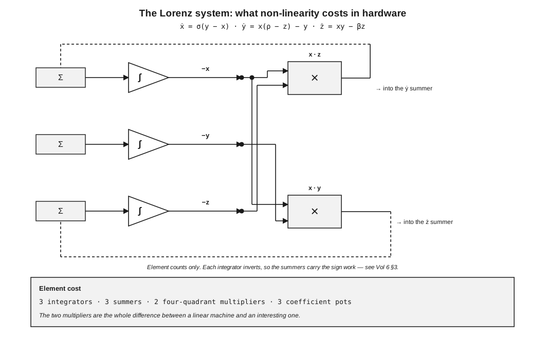
Figure 3 — The Lorenz system, showing element cost rather than full coefficient detail. Diagram authored for this dive by build/make_diagrams.py.

The Lorenz system is the standard demonstration of a homebrew machine, and it was the first program Fitch ran:

$$\dot{x} = \sigma(y - x) \qquad \dot{y} = x(\rho - z) - y \qquad \dot{z} = xy - \beta z$$

Three features make it a good test of everything in this volume.

It needs three integrators and two multipliers. One for each state variable, and the products $xz$ and $xy$. This is the element cost of non-linearity, and it is why Vol 2 §6 treats the multiplier as the element that decides whether a machine is interesting.

The multiplier’s internal scaling enters the coefficients. An AD633 computes $XY/10$ (Vol 2 §6.1). That factor of ten is not an inconvenience but a scaling aid: it is precisely what keeps the product of two full-scale variables inside one machine unit. The programmer must nevertheless carry it explicitly, because a coefficient derived without it will be wrong by a factor of ten.

The variables have very different ranges. In the classical parameter set, $z$ occupies a range roughly twice that of $x$ and $y$ and, unlike them, is not centred on zero. Applying one scale factor to all three either overloads $z$ or wastes most of the range on $x$ and $y$. This is the case where step 2 of Figure 1 cannot be skipped.

The multiplier is the accuracy budget. With a guaranteed 2 % of full-scale error (Vol 2 §6.1), no amount of care elsewhere makes this program accurate. What it will do faithfully is reproduce the qualitative behaviour — which is the entire point of running it, and a fair illustration of where analog computation is strong.

---

6.7 Static Check-Out

This is the procedure that separates an answer from a picture, and it is the step most often skipped.

6.7.1 The Principle

Before the machine runs, every amplifier output is a computable number. With the machine held in IC, the integrator outputs are the initial conditions, and every summer and inverter output is determined by them and by the coefficient settings. All of these can be predicted on paper from the flow diagram and then measured.

A disagreement at this stage is a patch error, a pot error or a wiring error — never a dynamics problem. That is what makes the check valuable: it isolates the entire class of setup mistakes before any dynamic behaviour can disguise them.

6.7.2 The Procedure

1. Patch the program and set every coefficient, measuring rather than reading dials (Vol 3 §6.2).
2. Select IC and apply the initial conditions.
3. From the flow diagram, predict the output of every element. Write the predictions on the diagram.
4. Measure every element output in turn. Investigate any disagreement beyond the machine’s expected tolerance.
5. Only then select OP.

6.7.3 The Dynamic Checks

Once static check-out passes, three further checks catch errors it cannot:

Table 6 — Once static check-out passes, three further checks catch errors it cannot

Check	Method	Catches
Known solution	Run a case with an analytic answer — an undamped oscillator should have constant amplitude, a first-order lag should reach 63 % in one time constant	Coefficient and scale-factor errors
Halve the time scale	Double every integrating capacitor; the solution shape must be identical and twice as slow	Errors in anything that is not an integrator, since only the integrators should respond
Parameter sweep	Vary one coefficient across its range and confirm the qualitative behaviour changes as theory predicts — a damping coefficient through zero should pass from decay to growth	Sign errors and misidentified inputs

The second is particularly good value, because almost any patching error produces a solution that does not simply slow down when the capacitors change.

---

6.8 Troubleshooting

Table 7 — Troubleshooting

Symptom	Most likely cause	Next check
Output grows exponentially on a problem that should decay	Sign error in a feedback path — typically the §4.4 case, feedback taken before the inverter rather than after	Trace the sign around the loop element by element
Solution is right in shape, inverted in phase	Initial-condition polarity	Check which integrator output the IC is set on
Solution correct at low rates, wrong when sped up	Reset not completing before OP begins	Vol 3 §2.3 — compute $7R_{IC}C$ and compare with the reset interval
Solution drifts steadily with no input	Integrator offset untrimmed, or leakage across the shorting switch	Vol 3 §5 — balance first, then investigate the switch
Amplitude flattens at the peaks	Overload — the amplifier is clipping and the equation has stopped holding	Rescale; do not adjust coefficients to compensate
Answer changes between otherwise identical runs	Dielectric absorption in the integrating capacitor, or an initial condition that has not settled	Vol 3 §4
Everything is slightly wrong in the same direction	Reference error, or a drop along the reference distribution	Vol 5 §7.3
One coefficient behaves as though it were different from its dial	Potentiometer loading	Vol 2 §5 — set it by measurement under load

The first row is the most common error in analog programming and the last two are the most commonly misdiagnosed.

---

6.9 The Discipline in One Page

1. Solve for the highest derivative and draw the flow diagram from it, literally.
2. Estimate every maximum; scale so the expected peak is 0.5 to 0.9 of full scale.
3. Rewrite each coefficient in scaled variables; realise it as pot × input weight.
4. Resolve the signs by tracing the loop, remembering that each amplifier inverts and no potentiometer can be negative.
5. Choose $\beta$ from the readout, and change it by changing every capacitor together.
6. Check statically against the diagram before believing anything.
7. Confirm with a known solution and a time-scale change.
8. Keep the diagram. It is the only copy of the program.

---

6.10 What Comes Next

Vol 7 closes the series: the licence position of every design surveyed, set out in full; where the modern reimplementations genuinely depart from the 1960s machines and where they only appear to; and the open questions this dive could not settle.