Homebrew & Open-Source Analog Computers — Volume 3 — Integrators, mode control and what is genuinely hard

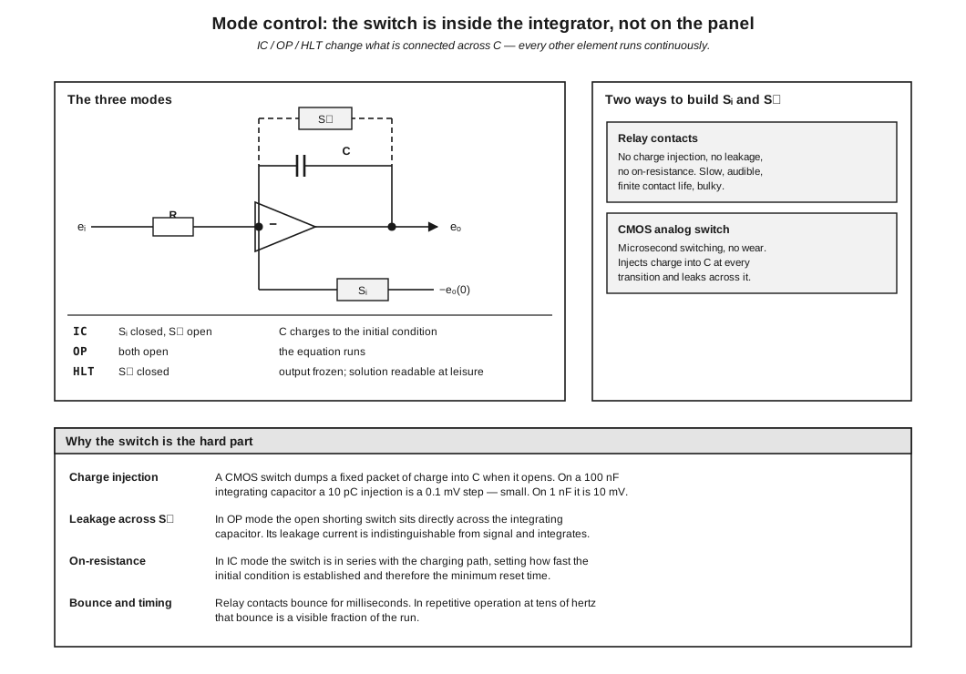
Figure 1 — Mode control and its error mechanisms. The switches that select IC, OP and HLT sit inside each integrator, across and around the integrating capacitor; nothing else in the machine is switched. Diagram authored for this dive by build/make_diagrams.py.

---

3.1 About This Volume

Vol 2 treated six kinds of computing element and found five of them straightforward. This volume is about the sixth.

An integrator is a summing amplifier with a capacitor in the feedback path, which is trivial. An integrator that can be set to a starting value, released at a defined instant, frozen on demand, and reset to run again is not trivial, and the difference is where homebrew machines fail. The circuit that does this is three switches and a capacitor, and each of the four things in that sentence has a failure mode that silently corrupts the answer rather than stopping the machine.

The volume also covers the diagnostics that make those failures visible — overload detection and static check-out — because homebrew designs omit them more often than not, and a machine that cannot tell the operator it has overloaded is a machine that will lie convincingly.

Cross-references: Vol 2 §4 for the integrator transfer function and drift terms; Vol 4 for what each documented design actually built; Vol 6 §5 for the check-out procedure that uses the diagnostics described here.

---

3.2 The Mode Problem

3.2.1 Why the Switch Is Inside the Integrator

A patched analog computer is a continuous circuit. Every summer, inverter, multiplier and potentiometer in it is running all the time, and none of them has any notion of a run beginning or ending. Only the integrators have state, and that state lives in one place: the charge on the feedback capacitor.

It follows that controlling the machine means controlling the capacitors, and nothing else. The mode control does not gate signals, does not disconnect the patch field and does not start or stop anything. It manipulates what is connected across and into each integrating capacitor, simultaneously, across every integrator in the machine.

This has a consequence homebrew designers regularly discover late: the mode control is not a panel switch, it is a bus. Every integrator needs the control signal, the signal must reach them all at the same instant, and adding an integrator means extending the bus. A design that treats mode control as a front-panel toggle wired to one integrator does not scale to the second one.

3.2.2 The Three Modes

Table 1 — The Three Modes

Mode	Common names	Switch state	What the capacitor is doing
IC	Initial Condition, Reset, Set	IC switch closed, shorting switch open	Charging to the initial value through the IC network
OP	Operate, Compute	Both open	Integrating the summed input currents — the run
HLT	Hold, Halt	Shorting switch closed	Frozen; output holds its value for readout

Machines differ in whether HLT shorts the capacitor’s charging path or opens the input path; both freeze the output, with different leakage consequences. Fitch’s 2010 panel labels the three positions plainly as reset / compute / hold, which is the clearest naming in the surveyed record.

3.2.3 Reset Time

The IC mode has to finish before the run starts, and how long it takes is set by the charging path. With an IC network resistance $R_{IC}$ and capacitor $C$, the capacitor settles exponentially with time constant $R_{IC}C$, and reaching 0.1 % of the target takes about seven time constants.

This is worth an arithmetic check because it constrains repetitive operation directly. With $C = 100$ nF and a 100 kΩ IC network, the time constant is 10 ms and settling to 0.1 % takes roughly 70 ms — which means a repetitive rate above about 10 Hz will begin each run before the initial condition has arrived. A machine whose repetitive solutions look subtly wrong at high rates and correct at low rates is usually exhibiting exactly this, and the symptom is easily misread as an amplifier problem.

The commercial reference point is useful here: the Heathkit EC-1 offered repetitive operation from 0.1 to 15 Hz, and THE ANALOG THING provides an OP-TIME control alongside its mode switch precisely so the run length and the reset can be reconciled.

---

3.3 Implementing the Switches

3.3.1 Relays

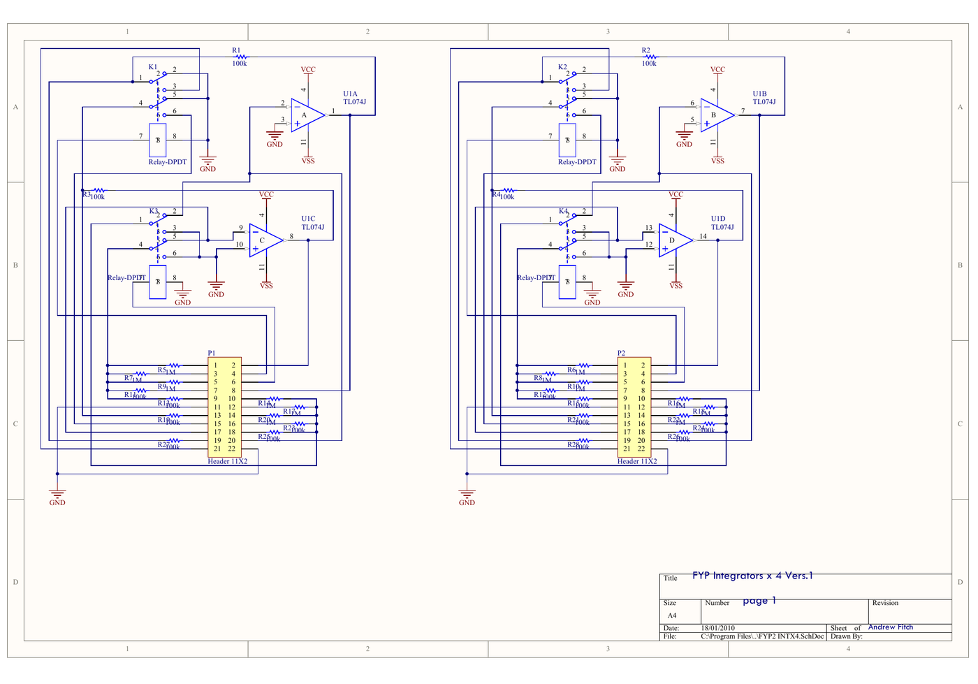
Figure 2 — Four relay-switched integrators, sheet 1 of 3 of Fitch’s 2010 design. Each of the four TL074 sections has its own DPDT relay (K1–K4) handling both the shorting and initial-condition paths; the 1 MΩ and 100 kΩ input resistors give the weight-1 and weight-10 inputs, brought out to the panel through 11×2 headers. Design document held locally; provenance and licence status in photo_credits.txt.

The relay is the oldest answer and remains a good one. It offers a genuinely open circuit when open and a genuinely closed one when closed, with no charge injection, no leakage worth measuring and no on-resistance worth measuring. For an integrator, where the capacitor faithfully accumulates whatever error is presented to it, those three properties are worth a great deal.

Fitch’s design commits to relays completely: four DPDT relays, one per integrator channel, listed in the project bill of materials as Relay-DPDT in a DIP-16 footprint with designators K1–K4. The board carries a dedicated µA78M12CKC regulator producing a 12 V rail for the relay coils, separate from the ±15 V analog supply — a detail visible on the third schematic sheet under the heading “12V FOR RELAYS”, and a sound one, because coil current transients have no business on the rails feeding the computing amplifiers.

The costs are equally real:

Table 2 — The costs are equally real

Cost	Consequence
Contact bounce	Milliseconds of indeterminate state at every transition. At repetitive rates of tens of hertz this is a visible fraction of the run
Switching speed	Operate and release times in the millisecond range set a floor under the reset interval
Contact life	Finite. A machine in repetitive operation at 10 Hz accumulates 36,000 operations an hour
Coil drive	Every integrator needs a driver, a supply and a flyback diode
Audibility and size	A twenty-integrator machine clatters, and the relays dominate the board area

3.3.2 CMOS Analog Switches

The modern alternative replaces each contact with a CMOS transmission gate. Switching is in microseconds, there is no wear, no coil, no driver and no noise. The penalties are the three parameters relays do not have.

Charge injection is the one that matters most. When a CMOS switch turns off, the charge stored in its channel is dumped into the surrounding circuit, and for the shorting switch that means directly into the integrating capacitor. The resulting output step is $Q/C$, and the following table is derived from that relation for a representative 10 pC injection:

Table 3 — Charge injection is the one that matters most. When a CMOS switch turns off, the charge stored in its channel is dumped into the surrounding circuit, and for the shorting switch that means directly into the integrating capacitor. The resulting output step is $Q/C$, and the following table is derived from that relation for a representative 10 pC injection

$C$	Output step from 10 pC	As a fraction of a 10 V machine unit
1 µF	10 µV	0.0001 %
100 nF	100 µV	0.001 %
10 nF	1 mV	0.01 %
1 nF	10 mV	0.1 %

The pattern is the important part, not the specific figures: charge injection is negligible on a slow machine and becomes a first-order error on a fast one. A builder who speeds a machine up by reducing $C$ — the standard move, and the one Fitch’s own notes describe when going from 0.1 µF to 0.001 µF capacitors to see the Lorenz attractor properly — is simultaneously making charge injection a hundred times worse. The injected charge appears at the start of every run, so it presents as an initial-condition error that scales with nothing the operator set.

Note — The 10 pC figure above is a round number chosen to make the scaling visible, not a specification of any particular device. Charge injection varies by an order of magnitude across switch families and is a function of supply voltage and signal level. The figure for a chosen part must be taken from its own datasheet; none was verified for this dive.

Leakage is the second penalty and the more insidious one, because it acts throughout the run rather than at its edges. In OP mode the open shorting switch sits directly across the integrating capacitor, and its off-state leakage current is indistinguishable from signal current. It integrates, exactly like the amplifier’s bias current in Vol 2 §4.3, and adds to the same budget.

On-resistance is the third and the least troublesome. It appears in series with the IC charging path, lengthening the reset time computed in §2.3, and in series with any signal path it switches.

3.3.3 Choosing Between Them

Table 4 — Choosing Between Them

If the machine is…	Use	Because
Slow, human-timescale, $C \geq 100$ nF	Relays	Charge injection would be negligible anyway, and relays give a genuinely ideal switch for nothing
Repetitive, oscilloscope-rate, small $C$	CMOS switches	Relay bounce and contact life become disqualifying long before charge injection does
Both, switchable	Relays for IC, CMOS for HLT	The IC path tolerates milliseconds; the hold transition is the timing-critical one

The surveyed designs split cleanly on this and along the expected lines: the 1978 Practical Electronics machine and Fitch’s 2010 machine both use relays; THE ANALOG THING, which offers repetitive modes on its mode switch, does not.

---

3.4 The Capacitor

The integrating capacitor is the only component in the machine whose own physics enters the answer. Three properties matter, in this order.

Dielectric absorption is the dominant one and the least familiar. A real capacitor does not fully discharge when shorted: some charge is absorbed into the dielectric and returns afterwards. For an integrator this is precisely the wrong behaviour, because the machine shorts the capacitor at every reset and then expects it to start from a known state. The recovered charge appears as a run-to-run initial-condition error that depends on what the previous run did — a memory of the last solution contaminating the next one.

The ranking of dielectrics by dielectric absorption is well established and consistent across sources: polystyrene and polypropylene are the best practical choices, polyester and metallised film are noticeably worse, class-II ceramics such as X7R are much worse again, and electrolytics are unusable. That ordering is safe to act on.

Note — Specific dielectric-absorption percentages are widely quoted for each dielectric class, but no datasheet establishing them was consulted for this dive, and published figures vary by measurement method. The ordering above is stated without numbers deliberately. A builder should take the figure from the datasheet of the part actually chosen.

The commercial machines took this seriously — the EAI TR-10 specified polystyrene integrating capacitors held to ±0.1 % — and it is one of the clearest places where a homebrew machine can match professional performance cheaply, because the right dielectric costs very little at the capacitance values involved.

Leakage matters for the same reason the switch’s leakage does: any current into the capacitor integrates. Tolerance and stability matter least, because an integrator’s gain error from capacitor tolerance is a single scale factor the programmer can absorb into a coefficient, whereas the other two errors cannot be calibrated out.

Fitch’s design brings the capacitors out to the panel as patchable elements — 0.01 µF, 0.1 µF and 1.0 µF, with the integrator’s own 0.1 and 1.0 positions selectable — which puts the time-scale decision in the operator’s hands at the cost of routing the most sensitive node in the machine through a patch cord and two jacks. Vol 5 §4 returns to that trade.

---

3.5 The Drift Budget

Gathering the terms from this volume and Vol 2 §4.3, an integrator’s output drifts at a rate that is the sum of:

Table 5 — Gathering the terms from this volume and Vol 2 §4.3, an integrator's output drifts at a rate that is the sum of

Source	Contribution	Scales with
Amplifier input offset voltage	$V_{OS}/(RC)$	The product $RC$
Amplifier input bias current	$I_B/C$	$C$ alone
Shorting-switch off-state leakage	$I_{leak}/C$	$C$ alone
Capacitor leakage	$I_{leak}/C$	$C$ alone
Charge injection at mode transitions	$Q/C$, once per transition	$C$ alone, and is a step rather than a rate

Two design rules follow directly and are worth stating flatly:

Trim the offset. It is the largest term in every configuration examined in Vol 2 §7.2, and it is the only one that can be removed entirely with a potentiometer. A per-amplifier balance control is not a luxury feature; its absence is the single commonest gap in homebrew designs.

Having trimmed it, prefer a large $C$ and a large $R$. Every remaining term except the offset term improves with larger $C$, and the offset term depends only on the product. A machine built around 1 µF and 1 MΩ has a materially better error budget than one built around 10 nF and 100 MΩ, at the same time constant — with the caveat that large-value capacitors in good dielectrics are physically large, which is why fast machines exist at all.

---

3.6 The Diagnostics Homebrew Machines Omit

3.6.1 Overload Detection

An analog computer that overloads does not stop. The amplifier clips, the equation it was implementing silently ceases to hold, and the machine continues to produce a smooth, plausible, continuous curve that is not the solution. There is no error state and nothing on the panel changes.

This is the defining failure mode of the whole technology and the reason every serious commercial machine carries per-amplifier overload indication. The EAI TR-10’s brochure is explicit that its individual overload indicator exists so that “programming errors can be located with minimum delay”, and it offered an audible alarm as well; the Comdyna GP-6 panel carries an OVLD lamp; the Analog Paradigm Model-1’s PS module includes over- and under-voltage and overload detection.

The homebrew record is much thinner. The 1978 Practical Electronics design is the notable exception, providing an overload warning circuit with comparators and LEDs across its ten amplifiers — and its inclusion in an amateur constructional series is a fair indication of how necessary the author considered it. Most other surveyed designs provide nothing.

The circuit is not demanding: a window comparator on each amplifier output, tripping at some fraction of the rail above the machine unit, latched so that a momentary excursion is not missed, with a common alarm line. The cost is one comparator per amplifier. The alternative is a class of wrong answer that cannot be detected by looking at the result.

3.6.2 Coefficient Setting and Readout Without Patching

Reading a potentiometer’s dial gives its track position, not its coefficient, because the wiper is loaded by whatever it feeds (Vol 2 §5). Measuring the coefficient properly requires reference applied to the pot and the wiper measured under its actual load.

Commercial machines make this a mode: the operator selects a pot, presses a button, and adjusts against a null meter without moving a single patch cord. The Comdyna GP-6 devotes a front-panel address scheme and a digital voltmeter to it; THE ANALOG THING provides a COEFFICIENT selector and a display.

Homebrew machines generally do not, and the practical consequence is that setting a dozen coefficients becomes a dozen manual measurements with a hand-held meter, repeated whenever the program changes. Vol 6 §4 gives the procedure for a machine without the facility. A builder designing a new machine should regard a coefficient-readout path as a feature with a very high ratio of usefulness to parts count.

---

3.7 What the Documented Designs Actually Do

Table 6 — What the Documented Designs Actually Do

Design	Mode switching	Overload detection	Coefficient readout	Integrating capacitor
PEAC (1968)	Integrator mode switching provided in the base unit	Not established from the held material	Not established	Not established
Kronis (1978)	Relay-based Compute/Hold/Reset	Yes — comparators and LEDs	Not established	Not established
Fitch (2010)	Four DPDT relays, one per integrator, on a dedicated 12 V rail	None provided	None provided	Patchable 0.01 / 0.1 / 1.0 µF
Malmö (2022)	Switch and button hardware present on the V2 board	Not established	Not established	Not established from the BOM
EEVblog “GK” (2012–)	Not established from the surveyed portion of the thread	Not established	Not established	Not established
THE ANALOG THING (2021)	MODE selector with IC, OP, HLT and repetitive positions, plus OP-TIME	Yes — OL indicator on the panel	Yes — COEFFICIENT selector and display	Fixed, with patchable additional capacitors

Note — “Not established” means exactly that: the material held in this project does not settle the point. Several of these designs may well provide the facility. The row is left honest rather than filled by inference from a photograph.

The pattern that does emerge is consistent with Vol 1 §5’s observation: the two entries with the most complete diagnostics are the magazine series written for readers who would have to debug it themselves, and the commercial product. The personal projects, which is to say the ones whose builder already knew what the machine was doing, provide the least.

---

3.8 What Comes Next

Vol 4 reads the six documented designs end to end as engineering decisions, including the ones this volume has only sampled. Vol 5 covers the physical substrate — chassis, panel, jacks and power — including where the integrating capacitor and its very sensitive summing junction should and should not be routed. Vol 6 is programming, and opens with the static check-out procedure that uses the overload and readout facilities discussed in §6.