Homebrew & Open-Source Analog Computers — Volume 2 — The computing elements

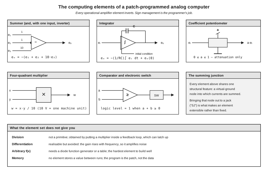
Figure 1 — The element set. Every operational-amplifier element inverts; sign management is the programmer’s work, not the machine’s. Diagram authored for this dive by build/make_diagrams.py.

---

2.1 About This Volume

A homebrew analog computer is an assembly of six kinds of thing. This volume takes them one at a time: what each must do mathematically, what limits its accuracy in practice, and which specific components meet the requirement.

The register here is deliberately concrete. This project has a documented history of authors inventing plausible component values, and the correction pass catching them. Every numeric specification in this volume is therefore attributed to the datasheet it came from, and every number that was calculated rather than read is labelled as a derivation and shown with its arithmetic. Where no source states a figure, that is said instead of estimated.

Vol 3 takes the integrator’s mode switch, which is the hardest element to build well and gets a volume of its own. Vol 4 reads the documented designs to see which of the choices below each one actually made.

---

2.2 The Operational Amplifier as a Computing Element

2.2.1 Why Everything Inverts

The computing amplifier is used in one configuration and one only: inverting, with the non-inverting input at ground. The signal enters through an input impedance to the inverting node, and a feedback impedance returns from the output to the same node.

Two properties make this the whole basis of the machine. First, negative feedback holds the inverting node at very nearly ground potential — the virtual ground, or, in the language every analog computer manual uses, the summing junction. Second, the amplifier’s input draws almost no current. Together these mean that the current arriving through each input impedance must leave through the feedback impedance, and that currents from different sources arriving at the same node do not interact.

That non-interaction is what makes the element set composable. Five sources can be wired to one summing junction and each contributes independently of the others. No other circuit topology gives this for free, which is why analog computers do not use non-inverting amplifiers for computing work even though it would save the inversions.

The cost is that every element changes the sign of its input, and the programmer has to track that. Vol 6 §3 treats the bookkeeping; Figure 1 above states the convention used throughout this series.

2.2.2 The General Relation

With input impedance $Z_i$ and feedback impedance $Z_f$, the output is $-,(Z_f/Z_i)$ times the input. Two choices of $Z_f$ produce the two elements that matter:

Table 1 — With input impedance $Zi$ and feedback impedance $Zf$, the output is $-\,(Zf/Zi)$ times the input. Two choices of $Zf$ produce the two elements that matter

$Z_f$	Element	Output
Resistor	Summer / inverter	Weighted, inverted sum of the inputs
Capacitor	Integrator	Inverted time integral of the weighted sum

Everything else in the machine either feeds these two or reads them.

---

2.3 The Summer and the Inverter

2.3.1 Transfer Function and Weighting

With several input resistors to one summing junction and a feedback resistor $R_f$, the output is the negated sum of each input scaled by $R_f/R_n$.

Homebrew designs almost universally provide two input weights, 1 and 10, by fitting input resistors of $R_f$ and $R_f/10$. Fitch’s 2010 machine does exactly this, as do the Malmö boards and THE Analog Thing. The reason is practical: a coefficient potentiometer can only attenuate, so a coefficient greater than one has to come from somewhere, and a gain-10 input is the cheapest place to get it. A programmer needing a coefficient of 3.5 uses a gain-10 input with the pot set to 0.35.

An inverter is a summer with one gain-1 input. It is not a separate circuit, and designs that list inverters separately from summers are describing panel provision, not topology.

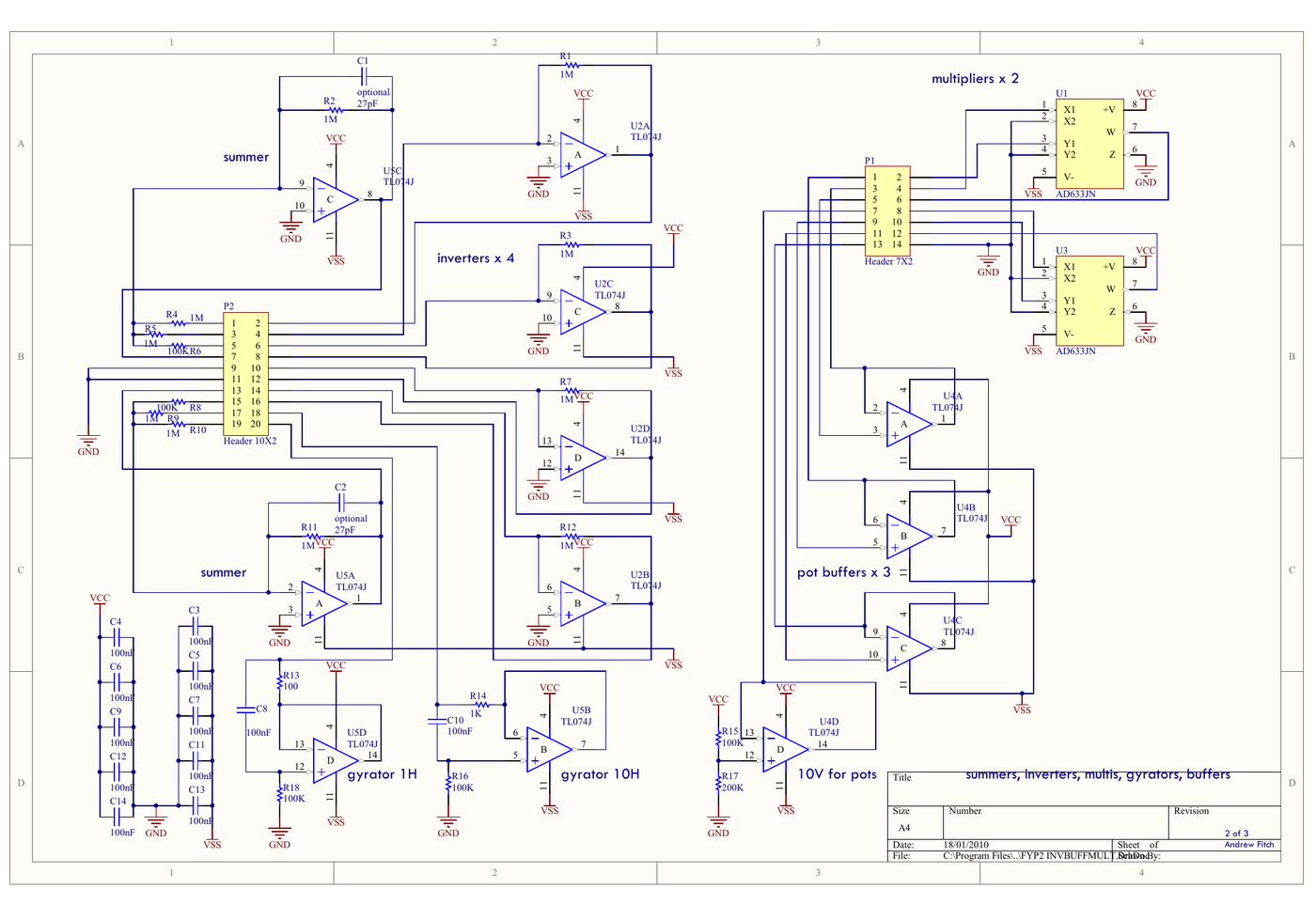
Figure 2 — The summer, inverter, multiplier, gyrator and buffer sheet from Fitch’s 2010 design, sheet 2 of 3. The summers use 1 MΩ feedback with 1 MΩ and 100 kΩ inputs, giving the standard weights of 1 and 10; note the 27 pF feedback capacitors marked “optional” across both summers. Design document held locally; provenance and licence status recorded in photo_credits.txt.

The detail worth noticing in Figure 2 is the pair of small capacitors marked optional across the summer feedback resistors. A summing junction with several patch cords landing on it accumulates stray capacitance, and that capacitance with the feedback resistor forms a phase lag that can make the amplifier ring or oscillate. A few tens of picofarads across the feedback resistor rolls the loop off before that happens. It is the kind of correction that appears in a real build and not in a textbook.

2.3.2 Where the Error Comes From

Three terms degrade a summer, in descending order of practical importance:

Table 2 — Three terms degrade a summer, in descending order of practical importance

Term	Effect	Mitigation
Resistor tolerance	Directly scales the coefficient. A 1 % resistor gives a 1 % coefficient error	Use 0.1 % metal film for the ratio-setting resistors; the absolute value matters much less than the match
Amplifier input offset voltage	Appears at the output multiplied by the noise gain; indistinguishable from a real input	Balance it out, or choose a part that does not have much — see §7
Finite open-loop gain	The summing junction is not exactly at ground, so the coefficient is slightly low	Negligible with any modern part; see the arithmetic below

The finite-gain error deserves one line of arithmetic because it is the term people worry about and it is the term that no longer matters. For a unity-gain inverter the fractional error is approximately $2/A_{OL}$. The TL074C datasheet specifies a minimum large-signal differential voltage amplification of 25 V/mV — that is, 25,000 — at ±15 V supplies with a 10 kΩ load.^[TL071/TL072/TL074 data sheet, Texas Instruments SLOS080W, September 1978, revised July 2025, §5.8 Electrical Characteristics (DC) for TL07xC.] That gives a worst-case gain error of about 0.008 %, which is an order of magnitude below the resistors. On the vacuum-tube machines this term dominated; on a transistor machine it has stopped being interesting.

---

2.4 The Integrator

2.4.1 Transfer Function

With input resistor $R$ and feedback capacitor $C$, the output is the negated integral of the input divided by $RC$, plus whatever the capacitor was charged to when the run began.

$RC$ is the integrator’s time constant and the single most consequential number in the machine. A machine with $RC = 1$ second solves problems on a human timescale, where a solution can be watched on a meter. A machine with $RC = 1$ millisecond solves the same problem a thousand times faster, which is what makes repetitive operation and a stable oscilloscope trace possible.

Practical designs make $C$ switchable to get both. Fitch’s panel offers 0.01 µF, 0.1 µF and 1.0 µF capacitors as patchable elements, and his own notes record the consequence directly: the first Lorenz run used 0.1 µF throughout and “runs a little slowly”, while a later version with 0.001 µF capacitors “runs much faster” and shows the attractor properly. That is the time-scale argument of Vol 6 §6 demonstrated on hardware rather than derived.

2.4.2 The Initial Condition

An integrator without a settable initial condition solves only the subset of problems that start at zero, which excludes most interesting ones. Every serious design therefore provides a path to charge $C$ to a chosen voltage before the run and to remove that path when the run starts.

That path, and the switch in it, is where homebrew machines are won and lost. It is the subject of Vol 3 and is not duplicated here.

2.4.3 The Two Drift Terms

An integrator integrates its own errors as faithfully as it integrates the signal. Two amplifier imperfections produce a steadily growing output with no input at all:

• Input offset voltage appears across $R$, driving a constant error current into the capacitor. Its contribution to the output drift rate is $V_{OS}/(RC)$.
• Input bias current flows into the capacitor directly. Its contribution is $I_B/C$.

Note the asymmetry: the offset term depends on the product $RC$, while the bias-current term depends on $C$ alone. A design that speeds the machine up by reducing $C$ makes the bias-current term worse while leaving the offset term unchanged if $R$ rises to compensate. This is the single most useful thing to understand about integrator part selection, and §7 works it numerically.

---

2.5 The Coefficient Potentiometer

A potentiometer across the reference, or across a signal, with its wiper feeding a summing junction, multiplies by a constant between 0 and 1. It cannot amplify. Every coefficient greater than unity must come from a gain-10 input, as §3.1 described.

Three practical points recur across the designs:

Table 3 — Three practical points recur across the designs

Point	Detail
Loading	The wiper feeds a finite input resistance, so the division is not the ratio of the track positions. The error is worst at mid-setting and vanishes at both ends. Designs either buffer the wiper or accept the error and set the pot by measurement rather than by dial reading
Resolution	A single-turn pot cannot be set to three figures by hand. Ten-turn precision potentiometers are the standard answer; Ulmann’s build of the Vogel design records having to fabricate spacers because the board material was too thin to hold them
Setting method	Reading a dial gives the track position, not the coefficient. Setting against a meter — with reference applied and the wiper measured — gives the coefficient. The commercial machines provide a dedicated mode for this; homebrew machines mostly do not, and Vol 6 §4 gives the manual procedure

Fitch’s design takes the buffering route explicitly: sheet 2 of his schematic set includes three amplifiers labelled “pot buffers”, plus a fourth generating the 10 V the pots work against.

---

2.6 The Multiplier

Multiplication of two variables is the element that separates a machine which can solve linear systems from one which can solve interesting ones. It is also the element homebrew builders almost never make themselves any more.

2.6.1 The Modern Answer

Since the 1980s the practical choice has been a monolithic four-quadrant multiplier, and in this field that overwhelmingly means the AD633. It appears in Fitch’s 2010 design (AD633JN), in the Malmö thesis machine (AD633JNZ), and in THE Analog Thing.

The datasheet figures that matter for computing work:^[AD633 Low Cost Analog Multiplier data sheet, Analog Devices, Rev. K, Features and General Description.]

Table 4 — The Modern Answer

Parameter	Value
Function	Four-quadrant, $W = XY/10$ with an internal laser-trimmed 10 V scaling reference
Total error	Within 2 % of full scale, laser-trimmed and guaranteed
Nonlinearity, Y input	Typically less than 0.1 %
Output noise	Typically less than 100 µV rms, 10 Hz to 10 kHz
Bandwidth	1 MHz; slew rate 20 V/µs
External components	None required

The 2 % figure is the one to hold onto. It is an order of magnitude worse than a well-built summer or integrator, and it means that in any program containing a multiplier, the multiplier is the accuracy budget. A builder agonising over 0.1 % resistors in the summers of a Lorenz patch is optimising the wrong element.

The internal division by 10 is not a quirk; it is what keeps the product inside the machine unit. Two variables at full scale would otherwise produce ten times full scale. Vol 6 §3 treats the scaling consequence.

2.6.2 What It Replaced

The AD633’s $1 self-containment should be read against what the earlier designs had to do. The 1978 Practical Electronics machine used two AD533JD multiplier ICs — the same idea, an earlier generation. The 1968 PEAC series devoted a whole optional unit to a four-quadrant multiplier built from discrete parts. The commercial machines of the same era used quarter-square multipliers built from matched diode networks, or, earlier still, servo-driven potentiometers. Vol 7 §4 treats this as one of the clearest places where the modern reimplementations depart from their ancestors: an element that was once a subsystem is now a single part costing less than the socket it sits in.

---

2.7 The Reference

The reference is easy to overlook because it computes nothing. It is nevertheless a computing element, because it defines the machine unit against which every coefficient, every initial condition and every constant term is expressed. An error in the reference is a multiplicative error in every number the machine produces.

Homebrew designs treat this with widely varying seriousness. Fitch’s design derives its pot supply from an op-amp fed by a resistive divider from the rails, and describes the three panel voltage sources as adjustable 0–10 V buffered outputs — adequate for chaotic-circuit work, where absolute accuracy is not the point. A machine intended to produce numbers needs a real reference device.

Where a precision reference is wanted, the part class is represented in this project’s own component library by the LT1236, whose datasheet specifies:^[LT1236 Precision Reference data sheet, Linear Technology, Features and Description.]

Table 5 — The Reference

Parameter	Value
Initial accuracy	0.05 % maximum
Temperature drift	5 ppm/°C maximum
Output	5 V and 10 V versions; sources and sinks up to 10 mA
Noise	Less than 1 ppm peak-to-peak, 0.1 Hz to 10 Hz
Ripple rejection	Greater than 100 dB
Minimum input/output differential	1 V

The sink capability in row three is the one that matters architecturally: an analog computer needs $+$ and $-$ reference of equal magnitude, and pots patched across the reference draw current in both directions as settings change.

---

2.8 Choosing the Amplifier: The Arithmetic

2.8.1 The Two Candidate Classes

Homebrew designs cluster on two very different parts, and the choice is usually made by availability rather than analysis. The comparison below uses only datasheet figures, cited, and then derives the consequence.

Table 6 — The Two Candidate Classes

Parameter	TL074C (JFET quad)	TL07xH (2020s revision)	OP07 (precision bipolar)
Input offset voltage, typ	3 mV	±1 mV	—
Input offset voltage, max at 25 °C	10 mV	±4 mV	75 µV
Offset drift	±18 µV/°C	±2 µV/°C	1.3 µV/°C max
Input bias current	65 pA typ, 200 pA max	±1 pA typ, ±120 pA max	±1.2 nA typ, ±4.0 nA max
Input offset current	5 pA typ, 100 pA max	±0.5 pA typ, ±120 pA max	0.5 nA typ, 3.8 nA max
Open-loop gain	25 V/mV min	118 dB typ	200–500 V/mV
Long-term stability	not specified	not specified	0.3 µV/month typ, 1.5 max
Channels	4	1 / 2 / 4	1

Sources: TL07x figures from Texas Instruments SLOS080W §5.7 (TL07xH) and §5.8 (TL07xC/AC/BC/I/M); OP07 figures from the Analog Devices OP07 data sheet, Features and Electrical Characteristics.

2.8.2 What Those Numbers Do to an Integrator

The following table is derived, not quoted. It applies $V_{OS}/(RC)$ and $I_B/C$ from §4.3 to the worst-case datasheet figures above, with $R = 1\ \text{M}\Omega$ throughout:

Table 7 — The following table is derived, not quoted. It applies $V{OS}/(RC)$ and $IB/C$ from §4.3 to the worst-case datasheet figures above, with $R = 1\ \text{M}\Omega$ throughout

$C$	$RC$	TL074C offset term	TL074C bias term	OP07 offset term	OP07 bias term
10 nF	10 ms	1 V/s	20 µV/s	7.5 mV/s	400 µV/s
100 nF	100 ms	100 mV/s	2 µV/s	750 µV/s	40 µV/s
1 µF	1 s	10 mV/s	0.2 µV/s	75 µV/s	4 µV/s

Three conclusions follow, and they are the practical content of this volume:

Untrimmed offset dominates everything. In every row, the offset term is two to four orders of magnitude larger than the bias-current term. Arguing about JFET versus bipolar input structures while leaving offset untrimmed is optimising the wrong parameter — which is why the commercial machines all provide a per-amplifier balance control, and why a homebrew machine without one is accepting a large, avoidable error.

Once offset is trimmed, drift takes over, and the parts separate sharply. Trimming removes the initial offset but not its temperature coefficient. Over a 10 °C change the TL074C contributes up to 180 µV of untrimmed offset against the OP07’s 13 µV — a factor of fourteen, and it recurs every time the room temperature moves.

The bias-current term is the one that punishes fast machines. At $C = 1\ \mu\text{F}$ the OP07’s bias current costs 4 µV/s, which is nothing. At $C = 10\ \text{nF}$ it costs 400 µV/s, twenty times the TL074C’s. A builder who speeds a machine up by reducing $C$ and keeps a bipolar amplifier has moved the dominant error term without noticing.

Note — None of this is a claim about measured machine accuracy. No homebrew design surveyed in Vol 1 §6 reports a measured error figure, and these derivations are upper bounds from worst-case datasheet limits, not predictions of what a given machine does.

2.8.3 Why the TL07x Family Persists Anyway

Given the table above, the TL074’s forty-year dominance in this field needs an explanation. It has four:

1. Four amplifiers in one package, which halves the board area of an element-dense design.
2. JFET inputs, giving picoamp bias currents that suit the large feedback resistances analog computers use.
3. It is everywhere and it is cheap, which for a one-off build matters more than a specification.
4. For chaotic and demonstration work the errors do not matter. A Lorenz attractor is qualitatively right with a 1 % element and qualitatively right with a 0.01 % one.

The fourth reason is the honest one for most of the record. It stops being sufficient the moment a machine is expected to produce a number rather than a picture — and that is precisely the boundary between the homebrew designs in Vol 4 and the commercial machines they are measured against.

---

2.9 How the Elements Reach the Panel

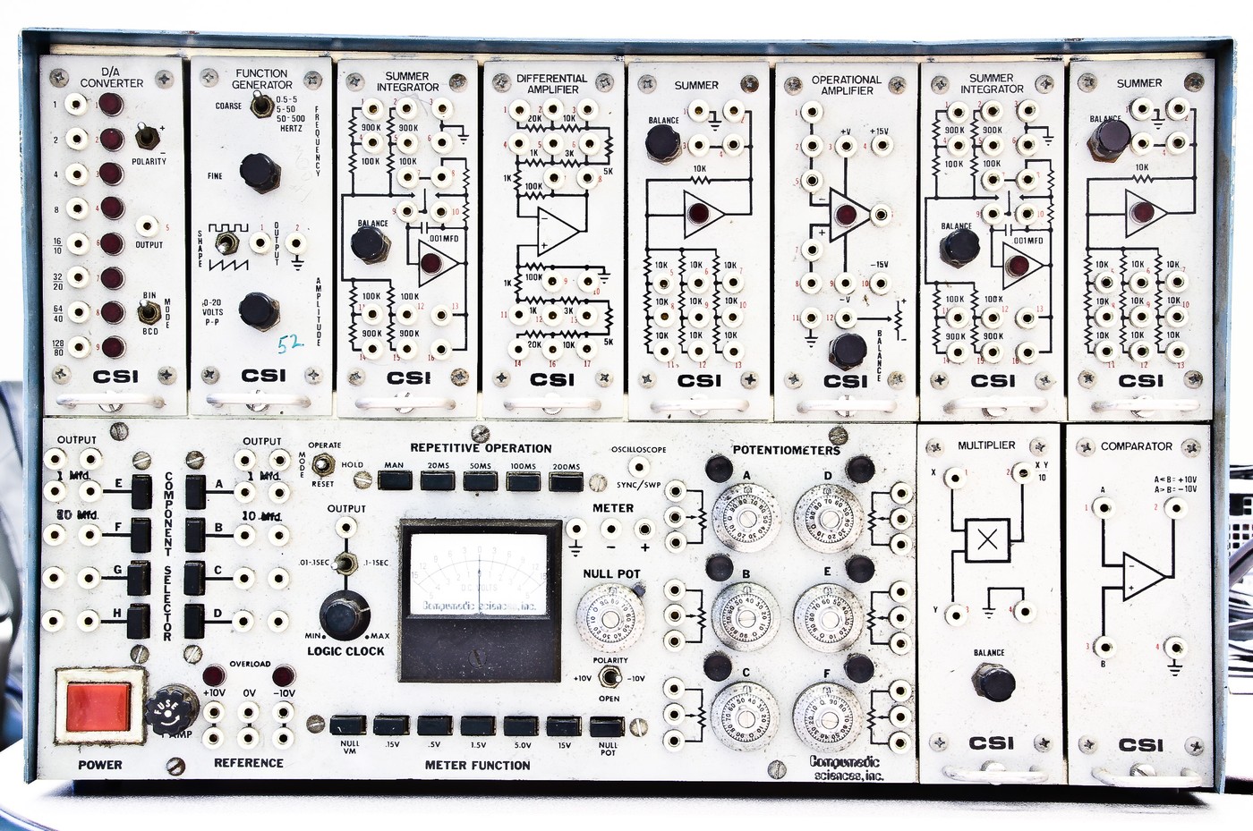
Figure 3 — Elements as panel surface, on a Computmedic Sciences 6F13 modular training machine. Each plug-in module’s face carries its own circuit diagram with the resistor values printed beside the jacks — 900 K and 100 K on the summer/integrators, 10 K ladders on the summer. Photograph held locally in this project; provenance is unrecorded and is discussed in photo_credits.txt.

Figure 3 shows the convention every good analog computer panel follows and most homebrew panels adopt: the panel is the documentation. The symbol printed around a group of jacks states what those jacks do, what weight each input carries, and where the summing junction is brought out. It cannot fall out of date because it is physically part of the thing it describes.

The homebrew designs in this series adopt this to varying degrees. Fitch’s panel (Vol 1 Figure 1) prints the amplifier triangles, the integration capacitor values and the gain weights directly into the artwork, with colour-coded rectangles grouping each element’s jacks. Vol 5 §4 treats panel and jack design as an engineering problem in its own right.

---

2.10 What Comes Next

Vol 3 takes the integrator’s mode switch — the IC/OP/HLT problem, charge injection, capacitor dielectric choice and the drift budget — which is the element that most sharply divides a machine that works from one that merely runs. Vol 4 reads the six documented designs to see which of this volume’s choices each one made, and what it cost them. Vol 6 returns to the element set from the programmer’s side, where the question is not what an integrator is but how many of them a given equation needs.