GE Project: Analog Computer EF-140 — Volume 5 — The mathematics the scales carry

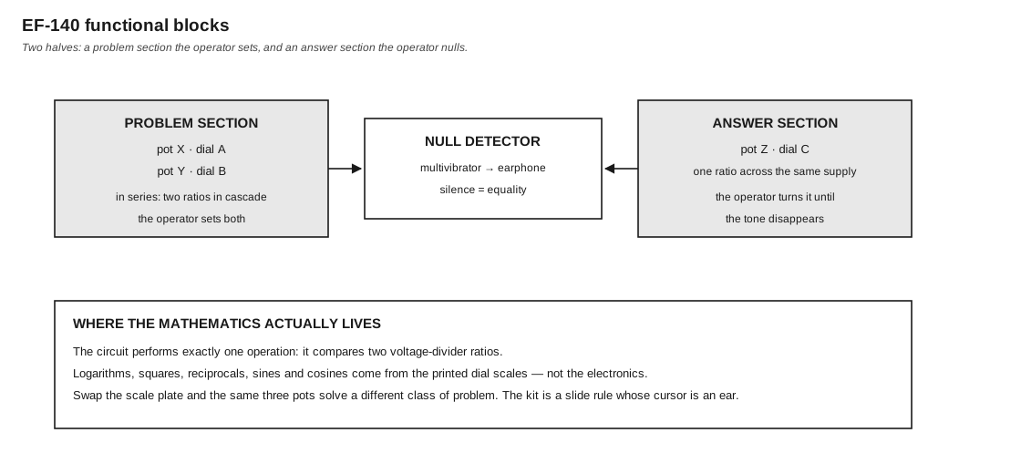
Figure 1 — Where the mathematics lives. The circuit compares two ratios and nothing else; every function beyond multiplication arrives on a printed card. Diagram authored for this dive.

5.1 About this Volume

Volume 2 established that the EF-140’s circuit performs exactly one operation: it compares two voltage-divider ratios. Volume 4 established that the operator’s job is to scale a problem into the range 0 to 1 and to restore the decimal point afterwards.

This volume covers what sits between those two facts — the printed scales. It works through the powers-of-ten discipline the machine demands, then each of the three scale plates in turn, checking General Electric’s own worked examples as it goes.

Several of those examples turn out to be considerably less accurate than the manual implies, and §4.4 says so with the arithmetic. That is not a complaint about a children’s kit; it is the clearest available evidence of where the machine’s real limits lie.

Cross-references: Vol 2 for the circuit; Vol 4 §4 for the scale plates as objects; Vol 6 for the problems that use these techniques; Vol 7 for what all of this implies about the machine’s class.

---

5.2 Everything Must Fit Between Zero and One

5.2.1 Why

A potentiometer’s wiper ratio k is bounded: 0 ≤ k < 1 (Vol 2 §3.2). The dials are therefore numbered 0 to 1.0 and nothing else will fit on them. The manual states the consequence immediately:

“Notice that the three scales are numbered only from 0 to 1.0. This means that a bit of number juggling will have to be done to deal with numbers larger than 1.0.”

This is the EF-140’s equivalent of amplitude scaling on an operational-amplifier machine, and it is the operator’s responsibility from beginning to end. The machine neither performs it nor checks it.

5.2.2 The Rule for Large Numbers

“Suppose you want to put 320 in power form. 320 has three digits. Move the decimal point three digits to the left, making it .320 or .32, and put a 3 as the exponent of 10. Thus, 320 = .32 × 10³.”

Count the digits, move the point that far left, and the count is the exponent. Mechanical and hard to get wrong.

5.2.3 The Rule for Small Numbers

“The negative exponent and the number of zeros between the decimal point and the first significant figure are the same. For instance, .00083 = .83 × 10⁻³.”

The manual is careful to distinguish this from the convention used in scientific notation proper, where “the negative exponent is one more than the number of zeros in front of the first significant figure” — its own example being the mass of a hydrogen atom, 6 × 10⁻²⁶, which for the machine becomes .6 × 10⁻²⁵.

Both statements are correct; they describe the same number in two normalisations. The machine’s normalisation puts the mantissa in [0.1, 1) so that it fits the dial; conventional scientific notation puts it in [1, 10). A reader moving between the manual and a physics textbook needs to keep the two apart, and the manual deserves credit for flagging it.

5.2.4 Recombining

Table 1 — 2.4 Recombining

Operation	Mantissas	Exponents
Multiplication	multiply on the machine	add
Division	divide on the machine	subtract

The manual’s summary for the awkward case: “with the scales on your computer, write down a number of zeros before the first significant figure equal to the negative exponent.”

5.2.5 The Worked Cases, Checked

Multiplication — 320 × 4200.

The manual: set dial X to .32, dial Y to .42, null, “the pointer will be at about .134”. Add the exponents, 3 + 4 = 7. Answer .134 × 10⁷ = 1,340,000.

Table 2 — 2.5 The Worked Cases, Checked

Machine reading	.134 → 1,340,000
True value	320 × 4200 = 1,344,000
Error	0.3 %

Correct to three figures as read, and the discrepancy is entirely in the third — exactly the “accurate to two places” the manual claims elsewhere. A well-behaved example.

Division — 498,000 ÷ 623.

The manual: rewrite as .498 × 10⁶ ÷ .623 × 10³; set .498 on scale C and .623 on scale B; null with dial X; read .8 on scale A; subtract exponents, 6 − 3 = 3; answer .8 × 10³ = 800.

Table 3 — 2.5 The Worked Cases, Checked

Machine reading	.8 → 800
True value	498,000 ÷ 623 = 799.4
Error	0.08 %

Also well behaved. Note that this example obeys the constraint the manual’s addendum later had to spell out — .498 is smaller than .623, so the null is reachable (Vol 4 §6.1).

A chained multiplication. The manual offers one genuine operating economy:

“At the end of each multiplication, when you read the answer on Scale C, transfer it immediately to scale A for the next multiplication. In that way, you can avoid having to write down any of the intermediate answers.”

The answer appears on dial Z and the next multiplicand goes on dial X, so a chain of products is a sequence of dial transfers with no paper in between. The exponents still have to be accumulated by hand.

---

5.3 Scale Plate No. 1 — Logarithms, Powers and Roots

5.3.1 The Scales

Plate 1 carries the linear scales A, B and C on the outside and the logarithmic scales D, E and F inside. The manual: “Notice that these scales are not equally spaced as are A, B, and C. They are logarithmic scales.”

5.3.2 The Idea

“Logarithms are powers. All logarithms used with your analog computer are ‘base 10’ logarithms, which means they are powers of the number 10. More exactly, the logarithm is the power to which 10 must be raised to equal that number.”

And the mechanism that makes logarithmic scales useful: “Logarithms are handy because they convert computation of powers and roots to simple multiplications and divisions.”

Since the machine multiplies, and since raising to a power is multiplying a logarithm, a logarithmic scale converts an operation the machine cannot do into one it can.

The manual demonstrates the scale correspondence physically: “Look at number 4 on scale D. Right next to it, on scale A, is .6, which is a close approximation of the log of 4 or 0.602.” The two scales are the same physical positions labelled two different ways — which is exactly what a logarithmic scale is.

5.3.3 Powers

The procedure: set the power on Scale A, the number on Scale E, null dial Z, read the logarithm of the answer on Scale C. Then interpret the logarithm: the digit left of the decimal point is the characteristic and gives the order of magnitude; the digits to the right are the mantissa and give the figures, recovered as an antilogarithm from Scale F.

The manual’s explanation of the characteristic is good:

“numbers between 1 and 10 have logs between 0 and 1.000; numbers between 10 and 100 have logs between 1.000 and 2.000; numbers between 100 and 1,000 have logs between 2.000 and 3.000… It is easy to remember that the answer will always be in three figures if the characteristic is 2, or in four figures if the characteristic is 3.”

5.3.4 Where the Accuracy Goes

This section checks the manual’s own examples. The arithmetic is this series’.

Square root of 4. Rewrite as 4^0.5 = .5 log 4. Set .5 on A, 4 on E, null, read the log on C: .3. Antilog of .3 on F: 2.

Table 4 — 3.4 Where the Accuracy Goes

Machine	2
True	2
Error	none

Exact, because log 4 = 0.602, half of it is 0.301, and the antilog of 0.301 is 2.00.

Cube root of 500. Set .33 on A, 5 on E, null, read .233 on C. Add log 100 ÷ 3 = .667. Total .900. Antilog: 8.

Table 5 — 3.4 Where the Accuracy Goes

Machine	8
True	7.937
Error	0.8 %

Good.

Three to the fifth power. Set .5 on A (the power 5 divided by 10), 3 on E, null, “read the log of the answer on scale C. It is approximately 0.23.” Multiply by 10: 2.3. Characteristic 2, mantissa .3, antilog 2, so “your final answer is approximately 200.”

Table 6 — 3.4 Where the Accuracy Goes

Machine	200
True	3⁵ = 243
Error	18 %

The manual presents this result without comment.

2500 to the fifth power. Set .5 on A, 2.5 on E (the number divided by 1000), null, “read the log of the answer on scale C. It is approximately 0.2.” Multiply by 10: 2.000. Mantissa zero, antilog 1, characteristic 2, so 100. Multiply back by (10³)⁵ = 10¹⁵. “So your final answer is approximately 100 × 10¹⁵ which is 10¹⁷.”

Table 7 — 3.4 Where the Accuracy Goes

Machine	1.0 × 10¹⁷
True	2500⁵ = 9.77 × 10¹⁶
Error	2.4 %

5.3.5 Why the Power Method Degrades

The 18 % error on 3⁵ is not a mistake in the manual; it is the method working as designed, and the reason is worth stating because it is a general property of logarithmic computation.

The machine reads a logarithm to two figures, then that logarithm is multiplied by ten, and only then converted back to a number. Multiplying the logarithm by ten multiplies its absolute error by ten as well. An error of 0.01 in a logarithm that is about to be scaled by ten becomes an error of 0.1 in the final logarithm — and an error of 0.1 in a logarithm is a factor of 1.26, or 26 %, in the answer.

The true value here is log 3 = 0.4771, so 0.5 × log 3 = 0.2386. The manual reads 0.23 — an error of 0.0086, which is entirely reasonable for a dial read to two places. Scaled by ten it becomes 2.30 instead of 2.386, and the antilog of that difference is the 18 %.

The practical rule: on this machine, powers and roots computed through the logarithmic scales are reliable to about one significant figure when the exponent is large, and to two when it is small. Roots behave far better than powers, because taking a root divides the logarithm and therefore shrinks the error rather than magnifying it — which is exactly what the square-root and cube-root examples above show.

Note — A reader taking the manual’s worked answers as demonstrations of the machine’s accuracy would be misled. The 3⁵ example demonstrates the machine’s procedure, not its precision, and General Electric’s failure to distinguish the two is the one genuine pedagogical weakness in an otherwise careful manual.

5.3.6 Negative Logarithms

Numbers below 1 have negative logarithms, and the manual handles them in the traditional way — as a positive mantissa with a negative characteristic written as a subtraction:

“For log .9, we write: 9.954 − 10. (If we wanted log .09, we would write 8.954 − 10, and so on.)”

The worked case is a radioactive-decay problem requiring (0.9)³:

3 log .9 = 3 (9.954 − 10) = 29.862 − 30

then, to bring it back to standard form, subtract 20 from both parts to give 9.862 − 10. Set .862 on scale C, read 7.2 on scale F; the characteristic 9 − 10 places the answer below 1, giving 0.72.

Table 8 — 3.6 Negative Logarithms

Machine	0.72
True	0.9³ = 0.729
Error	1.2 %

Correct. This is the most mathematically demanding technique in the manual, and it is presented to an audience that has just been told what a logarithm is.

---

5.4 Scale Plate No. 2 — Trigonometric Functions

5.4.1 Direct Reading

Plate 2 carries sine and cosine values for angles up to 90°, readable on any of the three dials:

“To find the sine of an angle of 20°, for example, set the pointer to 20 on scale D, E or F of Scale Plate No. 2, and read the answer directly on scales A, B or C. Sin 20° = .342”

Table 9 — 4.1 Direct Reading

Manual	.342
True	sin 20° = .3420
Error	none at three figures

This is not a computation at all — the machine is being used as a printed table, and the circuit is not involved. The dial is a look-up device.

5.4.2 Trigonometry Combined With Multiplication

The circuit re-enters when a trigonometric value is one factor of a product:

“For problems using sine and cosine functions, as .3 sin 37°, set the multiplier (.3) on scale A, the angle (37°) on the sin scale of dial Y, and adjust dial Z for null. The answer can be read on scale C: .3 sin 37° = .18”

Table 10 — 4.2 Trigonometry Combined With Multiplication

Manual	.18
True	.3 × .6018 = .1805
Error	0.3 %

Correct. The elegance here is that dial Y’s physical position encodes 37° on one scale and .6018 on another; the circuit multiplies the ratio regardless of which label the operator is reading.

5.4.3 Functions Not Printed

Tangent, cotangent, secant and cosecant are absent, and the manual explains why and what to do:

“To avoid burdening the dials, these are not indicated, but can be found by using trigonometric relationships on the memory board.”

Its example: cosec 30° = 1 / sin 30° = 1 / .5 = 2. Correct.

Angles beyond 90° are handled by a table on the memory board giving sine and cosine up to 360°, with the pragmatic note that “in most practical problems, the angles you deal with are acute angles.”

5.4.4 The Range Problem

The manual’s own worked ballistic example runs into a limit it does not name. Computing a gun’s range:

     V₀² sin 2A
R = ------------
         32

with V₀ = 3,000 ft/s and A = 30°, giving R = (9,000,000 × .866) / 32 = 7,794,000 / 32 = 243,562 ft. The manual states “The range is 240,000 feet.”

The arithmetic is right, but notice that the intermediate quantity 9,000,000 and the final 243,562 are both far outside the dials’ range. Every step has to be carried as a mantissa plus an exponent by the operator, on paper. The machine contributes one multiplication by .866 and one division by 32. Vol 6 §7 returns to how much of GE’s problem set is like this.

---

5.5 Scale Plate No. 3 — Squares and Reciprocals

5.5.1 The Purpose

“Scale Plate No. 3 has been especially designed to enable you to perform multiple operations without resetting your dials. Thus you can solve a great variety of problems more rapidly.”

The worked example is a mixed chain:

.3 × .8 × .5
------------  = ?
     .6

The procedure: set dial X to .3 on scale A and dial Y to .8 on scale B; null dial Z, which reads approximately .24. Reset dial Y to .6 on scale B and null dial X, which reads .4. Reset dial Y to .5, the last multiplier, and null dial Z; the final answer on scale C is .2.

Checking: .3 × .8 = .24; .24 ÷ .6 = .4; .4 × .5 = .2 ✓

The economy is that the running result never leaves the machine — each step’s answer is already sitting on a dial, and only one dial moves per operation.

5.5.2 The Reciprocal Scale

“These scales, you will notice, simply go backwards. They have been scaled so that multiplication can be performed instead of division, and vice versa.”

Reversing a scale converts k into something proportional to 1/k, so an operation the circuit performs as a division reads as a multiplication. The manual’s example: .4 × .7 × .3 computed with dial Y set on the reverse scale E for the final factor, reading the answer on scale A.

5.5.3 The Square Scale

“Scale D is also a special scale. It is useful in solving problems containing a squared term, such as the formula for the area of a circle. Set the radius of the circle on scale D (pot X automatically squares the radius, which can be read on scale A), set π on scale B and read the area on scale C.”

A scale compressed so that equal physical steps represent squares turns r into r² at the moment of setting. The area of a circle then becomes a single multiplication by π — one dial movement for a formula that would otherwise take two.

This is the clearest single illustration of the volume’s thesis. Squaring is performed by the printing on a card. No component was added, no wire moved; the scale does it.

---

5.6 What the Scales Reveal

5.6.1 The Machine Is a Printing Problem

Collecting the three plates:

Table 11 — Collecting the three plates

Capability	Where it comes from
Multiplication, division	the circuit (Vol 2 §4)
Powers, roots, logarithms	logarithmic scales, plate 1
Sine, cosine	trigonometric scales, plate 2
Tangent, cosecant, etc.	identities on the memory board
Squares	the square scale, plate 3
Reciprocals	the reversed scale, plate 3
Chained operations	scale arrangement, plate 3
Formulas, conversions	printed on the memory boards
Powers of ten	the operator, on paper

Exactly one row of that table involves the electronics.

5.6.2 What Follows

The machine is extensible without being modified. A fourth scale plate would have added capability for the cost of printing a card. The kit as sold was, in a real sense, unfinished by design.

An EF-140 without its plates is nearly useless. It will still null, and it will still multiply if the operator fits a linear scale of their own. Everything else is gone. Vol 4 §4.3 made this point about survival; here it is the mathematical statement of the same fact.

The operator does the hardest part. Scaling into the 0-to-1 range, tracking exponents, choosing which dial to null, applying identities from the memory board and restoring the decimal point are all human work, and they are where the errors occur. The machine performs one comparison and performs it well.

5.6.3 Accuracy by Operation

This series’ assessment, from the checks in §2.5, §3.4, §3.6 and §4.

Table 12 — 6.3 Accuracy by Operation

Operation	Typical accuracy	Limiting factor
Multiplication	2 figures, ~0.3 %	reading the dial
Division	2 figures, ~0.3 %	reading the dial; range constraint (Vol 4 §6.1)
Direct sine/cosine look-up	3 figures	printing of the scale; no circuit involved
Trig combined with a multiplier	2 figures	as multiplication
Square via the square scale	2 figures	printing of the scale
Roots	2 figures	logarithm error is divided — favourable
Powers with a large exponent	1 figure	logarithm error is multiplied — unfavourable (§3.5)

That last row is the one a user needs to know and the manual never says.

---

5.7 What Comes Next

Vol 6 works through the forty-nine problems General Electric set with these techniques — what they cover, what they reveal about the intended reader, and where the published answers do and do not check out. Vol 7 asks what all of this makes the EF-140, set against the operational-amplifier machines that share its name.