EAI PACE TR-10 — Volume 7 — Use, teaching and aftermath

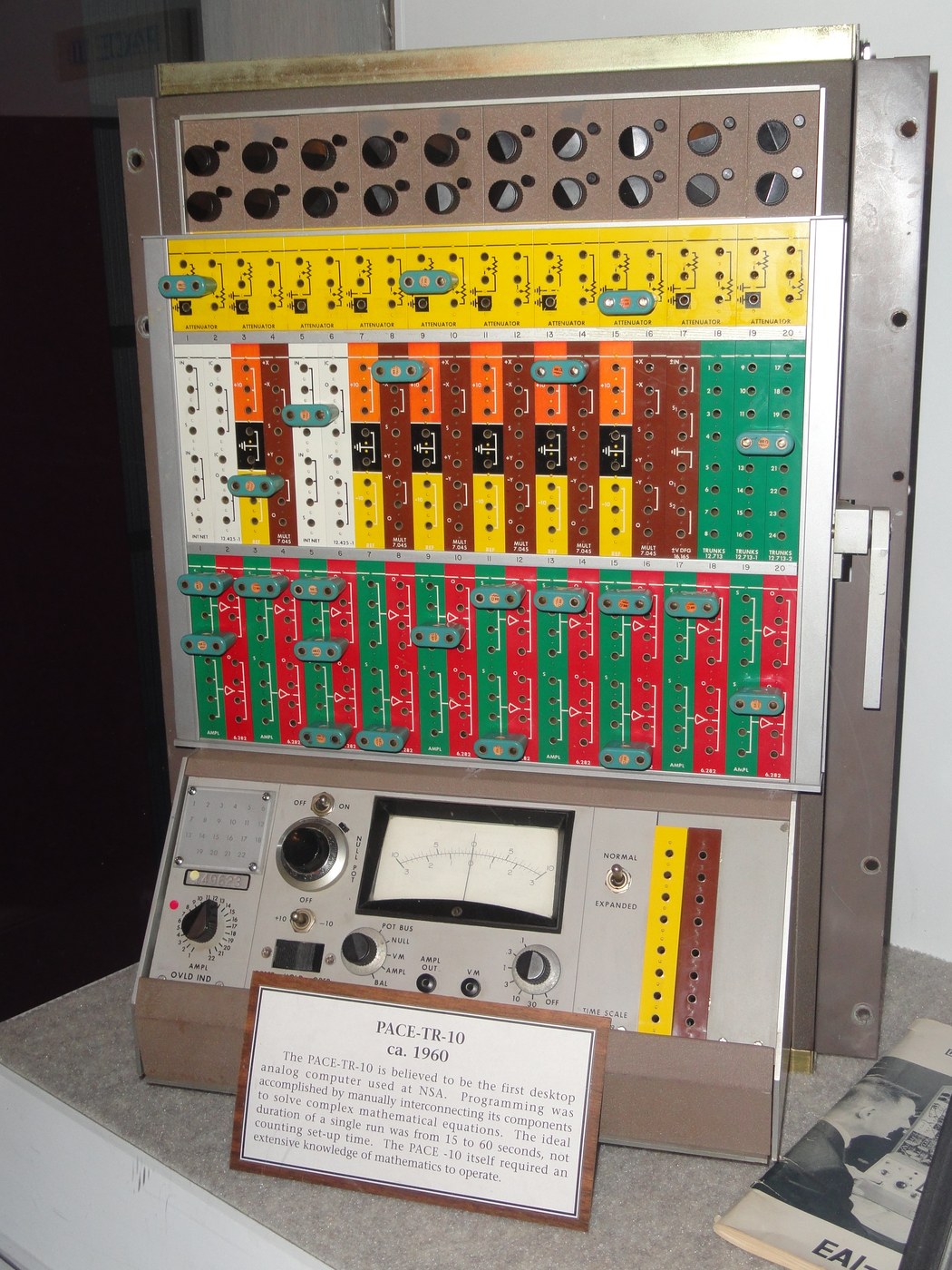
Figure 1 — A TR-10 as a museum object. The machine on display at the National Cryptologic Museum, complete in its console with attenuator, non-linear and amplifier rows filled. Photograph: File:PACE-TR-10 analog computer - National Cryptologic Museum - DSC07908.JPG by Daderot, CC0, via Wikimedia Commons.

7.1 About this Volume

The preceding six volumes described a machine. This one describes a practice.

It covers the working method EAI taught, what is known about who actually used TR-10s and for what, where the machine sat in a product line that was already turning away from pure analog computation while the TR-10 was still being sold, and what happened to the approach. It closes with what the machine is good for now.

More of this volume is inference and context than of any other, and the boundary is marked throughout. The direct evidence about TR-10 use held here amounts to one brochure page, one museum placard, and four dealer newsletters.

Cross-references: Vol 1 for sources and dating; Vol 4 for the programming method summarised in §2; Vol 6 for the documentary apparatus.

---

7.2 The Five Steps

EAI’s brochure lays out the working cycle in five photographs and five captions. It is worth taking seriously, because it is the only description held here of what an operator’s day actually looked like.

Table 1 — The Five Steps

Step	EAI’s caption
1 — Problem analysis	”Problem is translated into a mathematical description using algebraic and differential equations.”
2 — Programming	”An information flow sheet is prepared using a block diagram to represent the various computer elements and their interconnections.”
3 — Patching	”Following this diagram, the patch cord connections are made between the various computer elements.”
4 — Insertion of problem parameters	”Coefficient potentiometers are adjusted to provide design parameter inputs.”
5 — Solution	”The computer solution is performed in the exact manner prescribed by the mathematical equations. Solutions are presented on an XY plotter, strip chart recorder or on an oscillograph.”

7.2.1 What the Division of Labour Reveals

Three observations follow from the shape of that list.

Steps 1 and 2 happen on paper, away from the machine. The information flow sheet is the program. It is produced before any cord is touched, and it — not the patched console — is the artefact that gets filed, checked and reused. This is the compensation for the architectural fact established in Vol 2 §4.3: because the TR-10’s patch field is made of module faces and cannot be lifted out and stored, the paper has to carry the program. A TR-10 installation’s real library is a drawer of flow sheets.

Step 4 is separated from step 3. Patching defines the equation’s structure; pot settings supply its parameters. Separating them is what makes parameter studies cheap — the brochure’s whole pitch, “You simply turn a knob to feed in design parameters”, depends on structure and parameters being different operations. On a digital machine of the period both were a recompilation.

Step 5 names three output devices and no display. X-Y plotter, strip-chart recorder, oscillograph. The oscilloscope appears in the brochure’s photographs and in the repetitive-operation discussion, but EAI’s canonical output is paper. That is a real-time, one-solution-at-a-time working style, and it is the style the museum placard’s fifteen-to-sixty-second runs describe (Vol 5 §7).

7.2.2 The Skill Actually Required

The brochure claims the machine can be learned “as easily as you learned to use a slide rule”. The National Cryptologic Museum’s placard says it “required an extensive knowledge of mathematics to operate.”

Both are defensible about different things, and the difference is instructive. Operating a patched TR-10 — pressing RESET and OPERATE, turning a coefficient pot, reading the null meter — is genuinely easy. Programming one is not. Volume 4 showed what step 2 involves: rearranging an equation into highest-derivative form, choosing scale factors from estimated maxima, splitting each coefficient into a gain and a pot setting, and tracking a sign inversion through every amplifier. That is applied mathematics, and an error in it produces a plausible wrong curve rather than an error message.

The placard is the user site’s assessment and should be given more weight than the sales copy.

---

7.3 Who Used Them

7.3.1 The Direct Evidence

It is thin, and worth stating exactly.

One documented installation. The National Cryptologic Museum’s placard states that the TR-10 “is believed to be the first desktop analog computer used at NSA.” The hedge is the museum’s own. This establishes one agency, one machine, and an institutional recollection of how it was run.

One documented European distributor. EAI Electronic Associates GmbH of Aachen, whose dealer newsletters of 1965–66 are held here in translation. Newsletter no. 1 (July 1965) announces EAI’s “new exclusive distributorship for Germany” and offers the TR-10 integrator modification (Vol 5 §6) — evidence of an installed base in Germany large enough to justify a published field-modification procedure.

One surviving serial number. The console photographed for this series is serial no. 70, carrying a second plate reading model 45.009. Nothing follows from a single serial number about production volume.

Everything else in this section is the brochure’s account of its intended market, and is labelled as such.

7.3.2 The Market EAI Described

The brochure names three buyers, and they are worth separating because they wanted different things:

The individual engineer. “Because of its unique portability, this compact computer can become your personal tool… By allowing you to spend more of your time on creative engineering, it can enhance your value as an engineer.” The appeal is to time and autonomy — not waiting for someone else’s machine.

The organisation that already has a large installation. “Companies who already have large analog computer installations will find the PACE TR-10 can be used to solve smaller problems and eliminate tie-ups and excessive waiting time for large equipment.” The TR-10 as overflow capacity — the same economic argument that would later be made for the minicomputer against the mainframe, made here on the analog side several years earlier.

The training department. “It is ideal for breaking-in new engineers to the advantages and techniques of analog computation.” A machine cheap enough to let a novice make mistakes on.

7.3.3 What the Machine Was For

EAI’s own list of what the TR-10 addresses, from the repetitive-operation page, is the most specific statement of application held here:

• System optimisation — “the selection of parameter values which give the best overall performance”
• Boundary value problems — “the solution of differential equations in which the problem is to find the initial conditions for specified solutions of the equation”
• Model building — “the problem of determining a mathematical representation for a system of known response”
• Exploratory studies to conserve computing time, rapid approximation of optimum system parameters, determination of stability regions of control systems
• Integral transforms — Fourier integrals, superposition integrals, correlation functions
• Statistical studies requiring many solutions

Every one of these is a problem class where the same equation is solved repeatedly with different numbers, and where a fast approximate answer beats a slow exact one. That is precisely the shape of problem at which an analog machine with a repetitive mode is better than a contemporary digital machine — and precisely the shape at which it would later lose, once digital machines became fast enough that “repeatedly” stopped being expensive.

---

7.4 The Product Line Around It

The TR-10 was never a standalone product. The German newsletters, which mention it alongside its stablemates, allow the line to be sketched — and the sketch shows a company already moving.

7.4.1 The Desk-Top Family

Table 2 — 4.1 The Desk-Top Family

Machine	Appears in	Note
TR-10	newsletters 1, 2, 7 (1965–66)	the machine of this series
TR-20	newsletters 1, 2, 7	integrator networks type 12.1115 — the patch panel borrowed for the TR-10 modification (Vol 5 §6.3)
TR-48	newsletters 1, 2	expandable to a 58-amplifier configuration
TR-58	newsletters 1, 2	the expanded TR-48

Newsletter no. 1 details improvements to the TR-48/58 including “improved multipliers, variable-breakpoint function generators, delay-line and reactor-kinetics networks, fast comparators” — the same component vocabulary as the TR-10, one tier up.

The TR-10’s position in this family also explains the modification of Vol 5 §6: individual integrator mode control existed on the TR-20 and TR-48, and the field modification brings the TR-10 up to its siblings’ standard by transplanting a TR-20 patch panel.

7.4.2 The Turn to Hybrid

The newsletters are more interesting for what else they carry. By 1965–67 EAI’s German customer literature is not principally about analog computers.

Table 3 — 4.2 The Turn to Hybrid

Product	Newsletter	What it is
DES-30	no. 1 (1965)	digital extension system
PDS 1020	nos. 2, 7 (1965–66)	general-purpose digital computer, magnetostrictive delay-line memory
EMC	no. 2 (1965)	Electronic Mode Control upgrade for the TR-48/58
PC 12	no. 7 (1966)	process computer — used, the newsletter states, in the Surveyor Moon-landing mission
EAI 580	no. 12 (1967)	analog/hybrid: 80 amplifiers, 70 servo pots, ±10 V reference, ±0.01 % linear accuracy, built-in parallel logic, interfaces to the EAI 640 and the DEC PDP-8-S

Newsletter no. 12 also carries “a historical timeline of EAI analog and hybrid systems from 1948 to 1967” — a company narrating its own transition while it happened.

Two things stand out. First, the Electronic Mode Control option and the TR-10 integrator modification are the same idea: bringing mode switching under program control rather than under a human thumb. That is the analog machine reaching towards automation, and it is the direction hybrid computing came from. Second, by 1967 EAI’s flagship desk-top product is defined partly by which digital computers it connects to. The PDP-8-S appears in EAI’s own literature as a peer.

7.4.3 What Hybrid Meant

The hybrid machine is the honest answer to the analog/digital question of the period, and it is worth stating because it is where the TR-10’s lineage actually goes.

Analog hardware integrates continuously, in parallel, in real time, at a few tenths of a percent. Digital hardware stores programs, makes decisions, keeps results exactly, and repeats without drift. A hybrid system lets the analog side solve the differential equations while the digital side sets parameters, sequences runs, applies logic, and records results.

Everything the TR-10 offered as a manual facility has a hybrid counterpart: the coefficient potentiometer becomes a digitally set attenuator; the mode buttons become program-controlled mode lines — exactly what the 1965 modification exposed; the operator watching an oscilloscope and turning a knob becomes an optimisation loop. The German newsletter’s phrase for what the modification enables, “automatically operating iterative procedures”, is a description of hybrid operation written before the machine to do it had arrived.

---

7.5 The Displacement

7.5.1 What Actually Killed It

Analog computing did not lose because it was wrong. It lost on four specific counts, and it is worth being precise about them because the popular account — “digital was faster” — is the one thing that was not true for a long time.

Table 4 — 5.1 What Actually Killed It

Count	The analog position	Why digital won it
Accuracy	~0.1 % readout; components at 0.025 % to 0.4 %; errors accumulate along a chain	word length buys accuracy by the digit, and buys it uniformly
Program storage	the program is a patched console and a paper flow sheet	a program is data; it can be stored, copied, versioned, mailed
Reproducibility	pot settings drift, amplifiers need rebalancing, two runs differ slightly	identical inputs give bit-identical outputs, indefinitely
Generality	continuous systems only; no sorting, no text, no logic beyond a comparator	one machine for every problem

Speed is conspicuously absent. For real-time parallel solution of a system of coupled differential equations, the TR-10 was faster in 1960 than the digital machines it competed with, and remained so for years. What it could not do was keep the answer, repeat the answer, or be reused for anything that was not a differential equation.

7.5.2 The Economics of the Patch Cord

One underrated factor: setting up an analog problem is expensive in skilled human time and cheap in machine time; setting up a digital problem is the reverse. As machine time got cheaper every year and skilled engineering time did not, the balance moved steadily against the analog machine — independently of any technical comparison.

The museum placard’s remark that a run took fifteen to sixty seconds “not counting set-up time” is the whole economics in a parenthesis. The run was never the expensive part.

7.5.3 What Was Genuinely Lost

Two things, and both are still real.

Real-time parallel solution. Every amplifier in a TR-10 computes simultaneously and continuously. There is no timestep, no convergence criterion, no stiffness problem, and no question of whether the integrator is stable — the capacitor integrates exactly, in physics. For hardware-in-the-loop simulation this is not a stylistic preference; it is the requirement. The niche never disappeared, and it is the reason analog and mixed-signal techniques persist in specialised places.

The knob. The gap between changing a parameter and seeing the consequence was, on a TR-10 in repetitive mode, effectively zero. That immediacy shapes how a person builds intuition about a system, and it is qualitatively different from editing a number and re-running. Modern interactive simulation has recovered much of it, but it took decades, and it had to be rebuilt in software rather than being a free consequence of the hardware.

---

7.6 The Machine Now

7.6.1 What It Is Good For

As an object of study, the TR-10 is unusually clear. The architecture is legible from the front: every computing element is visible, labelled with its own function, and wired by hand into the equation being solved. A person who patches a second-order system on it and watches the damping change has understood something about differential equations that is genuinely hard to get any other way.

As a restoration project, it is harder than the Heathkit EC-1 and for an unexpected reason. The EC-1 is a vacuum-tube machine with a published schematic, and tubes, resistors and capacitors are replaceable. The TR-10 is a transistor machine with, as far as the record held here goes, no published schematic at all (Vol 6 §8). A failed module is a black box. The plug-in architecture that made it serviceable in 1960 — swap the module, diagnose later — depends on a supply of modules that no longer exists.

As a source of design ideas, several hold up: the module face that is also its own patch panel and its own documentation; the bus bar with a pull-out taper pin per component; the null-against-a-precision-pot readout that gets 0.1 % out of a 2 % meter; the individual overload indicator that converts a silent failure into a located one.

7.6.2 What to Do With One

Table 5 — 6.2 What to Do With One

If the machine is	Then
Complete and working	Patch the second-order program of Vol 4 §4 and run the parameter sweep. It exercises two integrators, three pots and the reference, and every number is published and checkable.
Complete but untested	Balance every amplifier and verify the ±10 V reference before anything else (Vol 4 §8). Those two account for most apparent faults.
Missing modules	Record what is present, by type number from the silkscreens, before anything is moved. The type numbers are the machine’s only self-documentation (Vol 3 §2.2).
A parts machine	Photograph every module face and every data plate first. A silkscreen photograph settling the 16.156-or-16.155 question (Vol 6 §5.3) would be a genuine contribution to the record.

7.6.3 The Documentary Gap

This series ends where it began. The TR-10 is a well-made, well-documented-at-the-time machine about which the surviving public record is thin, contradictory in places, and missing the one document — the maintenance manual — that would answer most remaining questions.

That is not unusual for equipment of this class. Sales literature survives because it was printed in quantity and looks attractive; maintenance manuals were printed in small numbers, went to service departments, and were thrown away when the product line ended. The asymmetry systematically biases what can be known about old machines towards what their makers wanted said about them.

The corrective is the one applied throughout these seven volumes: say which document each figure comes from, and say plainly when there is no document at all.

---

7.7 Summary

Table 6 — Summary

What it was	A fully transistorised, plug-in, desk-top general-purpose analog computer, in production by about 1960 and still supported in 1966
What it did	Solved ordinary differential equations in hardware, in parallel, in real time or up to 500 times faster
Who made it	Electronic Associates, Inc., Long Branch, New Jersey, under the PACE trade name
Its best idea	Capability as inventory: the console never changes, the modules decide what the machine is
Its real constraint	The program lives on paper, because the patch field cannot be removed
What is documented	Configuration, module specifications, two worked programs, repetitive-operation timing
What is not	Price, production, any schematic, the rep-op capacitor
Why it still matters	It is the clearest surviving demonstration of what was lost and gained when computation went digital