EAI PACE TR-10 — Volume 2 — System architecture

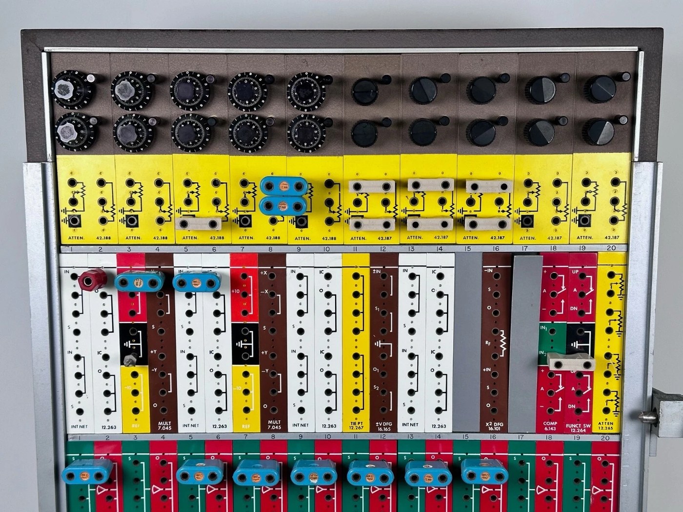
Figure 1 — The console face. The yellow strip across the upper cabinet is the attenuator row; the mixed white, brown and red modules below it are the non-linear row; the green-and-red band is the amplifier row. Every coloured face is the front of a plug-in module and every hole in it is a patching termination. Photograph: locally held collector image of serial no. 70.

2.1 About this Volume

Volume 1 described what the TR-10 is. This volume describes how it is put together: the division of the console into four areas that accept plug-in components, the rules governing what may be plugged where, the way power reaches every module, and the arrangement by which the machine’s patch panel is assembled out of the front faces of its own computing elements.

This is also the volume in which the two primary sources part company most seriously. The procurement specification requires one patching architecture; the brochure describes the machine as having a different one. Section 4 sets that out rather than quietly adopting whichever reading is more convenient.

Cross-references: Vol 1 for sources and dating; Vol 3 for what each module actually contains; Vol 4 for how a problem is laid onto this hardware; Vol 6 for the specification in full.

---

2.2 The Four Areas

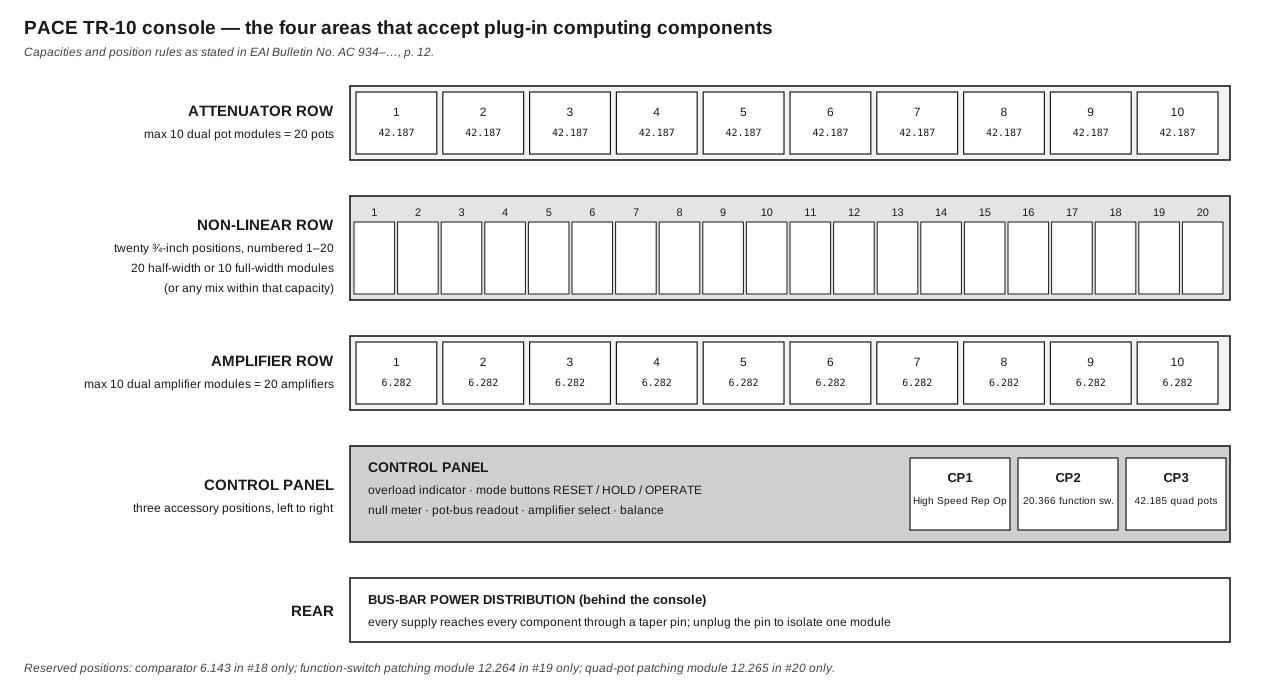
Figure 2 — Console architecture, drawn from the capacities and position rules stated on p. 12 of EAI Bulletin No. AC 934. Diagram authored for this dive.

2.2.1 The Division

The brochure states the division precisely: “That portion of the TR-10 Computer Console which accepts plug-in computing components is divided into four areas.” They are, from the top down:

Table 1 — The brochure states the division precisely: "That portion of the TR-10 Computer Console which accepts plug-in computing components is divided into four areas." They are, from the top down

Area	Position	Capacity
Attenuator row	top row	maximum of 10 Dual Coefficient Setting Potentiometer modules = 20 potentiometers
Non-linear row	middle row	twenty ¾-inch positions numbered 1–20; 20 half-width or 10 full-width modules, or any mix within that total
Amplifier row	bottom row	maximum of 10 Dual Operational Amplifier modules = 20 amplifiers
Control panel	right side of the inclined panel	three accessory positions, numbered CP1–CP3 left to right

The three control-panel positions are individually assigned rather than general-purpose:

Table 2 — The three control-panel positions are individually assigned rather than general-purpose

Position	Accepts
CP1	High Speed Repetitive Operation Control Panel
CP2	Type 20.366 Function Switch Assembly
CP3	Type 42.185 Quad Coefficient Setting Potentiometer Assembly

2.2.2 Half-Width and Full-Width

The non-linear row is the only one with a genuine packing problem, and the brochure spells out the geometry. Non-linear computing components are housed in full-width (1½ inch) or half-width (¾ inch) plug-in modules. The row consists of twenty ¾-inch positions, numbered across a strip at the top of the row to correspond with the module beneath.

A full-width module therefore occupies two adjacent odd-and-even position pairs — positions #1 and #2, #5 and #6, and so on. It is worth noting the consequence: a full-width module cannot straddle an even-odd boundary such as #2 and #3. The pairing is fixed by the console, not chosen by the operator.

2.2.3 Position Rules

Several module types are restricted, and three positions are effectively reserved. The rules as printed:

Table 3 — Several module types are restricted, and three positions are effectively reserved. The rules as printed

Component	Type	Permitted positions
Integrator networks	12.263 or 12.425	up to nine, in #1 through #18, each occupying an adjacent pair
Multipliers	7.045	up to nine, in #1 through #18, adjacent pairs (full-width module)
Variable DFG	16.154 / 16.156 / 16.165	any even-numbered position except #20
X² DFG	16.101	any even-numbered position except #20
Log DFG	16.126 / 16.133	any even-numbered position except #20
Reference panel	12.266	any even-numbered position except #20
Dual tie point panel	12.267	any position in the non-linear row
Comparator	6.143	#18 only
Function switch patching module	12.264	#19 only
Quad potentiometer patching module	12.265	#20 only

Two observations follow from the arithmetic. First, “up to nine” dual networks in eighteen positions is exactly consistent: nine dual modules at two positions each fill #1–#18, leaving #19 and #20 for the two reserved patching modules. The row’s capacity is not approximate; it is laid out to the position.

Second, the even-position-only rule for the function generators and reference panel is what makes the odd positions the “left half” of each full-width pair. The brochure closes the section with an escape clause worth recording:

“The above assignment of computing components applies to the standard TR-10 Console. Special computers may be supplied with provisions for mounting DFG’s or REFERENCE PANEL in the odd numbered positions (with the exception of position #1) or for accommodating more than one COMPARATOR.”

A surviving TR-10 that violates these rules is therefore not necessarily modified. It may be a special-order console.

---

2.3 The Plug-In Principle

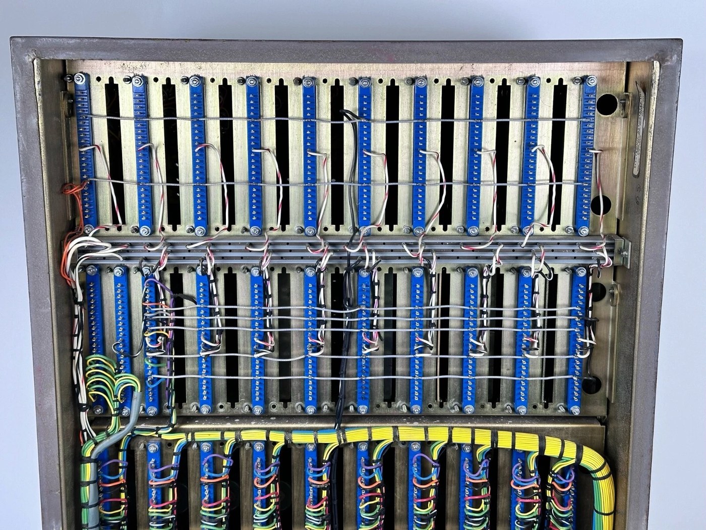
Figure 3 — The console from behind. Every module is retained by two nuts at the rear; the harness carries signal and supply lines to the fixed connectors that the modules plug into. Photograph: locally held collector image of serial no. 70.

2.3.1 Pre-Wired, Not Re-Wired

The design’s central claim is that the console arrives fully wired for its maximum complement, and that expansion is therefore purely mechanical. The brochure:

“The Basic Computer is completely wired to accept a full complement of computing components… Expansion of the computer to enable it to solve more complex problems is accomplished simply by plugging in the desired number and type of computing components… no additional wiring is necessary.”

The specification states the same requirement in its own register at §2.1: the computer “shall be pre-wired to accommodate up to twenty operational amplifiers and twenty-four precision potentiometers”, and “shall also be pre-wired to accept interchangeably” integrator networks, quarter-square multipliers, X² diode function generators, variable diode function generators, and log function generators.

2.3.2 Swapping a Module

The brochure illustrates the operation in four photographs, and the sequence is worth stating because it defines the machine’s service model:

1. At the rear of the console, remove the two retaining nuts that secure the component to be replaced.
2. Pull the component out of the computer — forwards, from the front face.
3. Plug the desired component into the empty position. No wiring is necessary.
4. Replace the retaining nuts and secure the component.

The brochure’s summary of step 4 is the whole argument in one sentence: “You effectively have a new computer.”

Specification §2.3 makes front-insertion a requirement rather than a convenience: “All computing components shall plug into the front of the computer to allow for quick and easy interchangeability, replacement and servicing.”

2.3.3 Servicing In Place

The Service Shelf, Type 51.039 completes the scheme. It is a shelf that “facilitates maintenance of any plug-in computing component under normal operating conditions” — that is, it allows a module to be withdrawn from its position and supported in front of the console while still connected and powered, so that it can be measured while the rest of the machine runs. A Service Shelf is part of the Standard Basic TR-10 complement, not an option.

---

2.4 The Patch Panel That Is Made of Module Faces

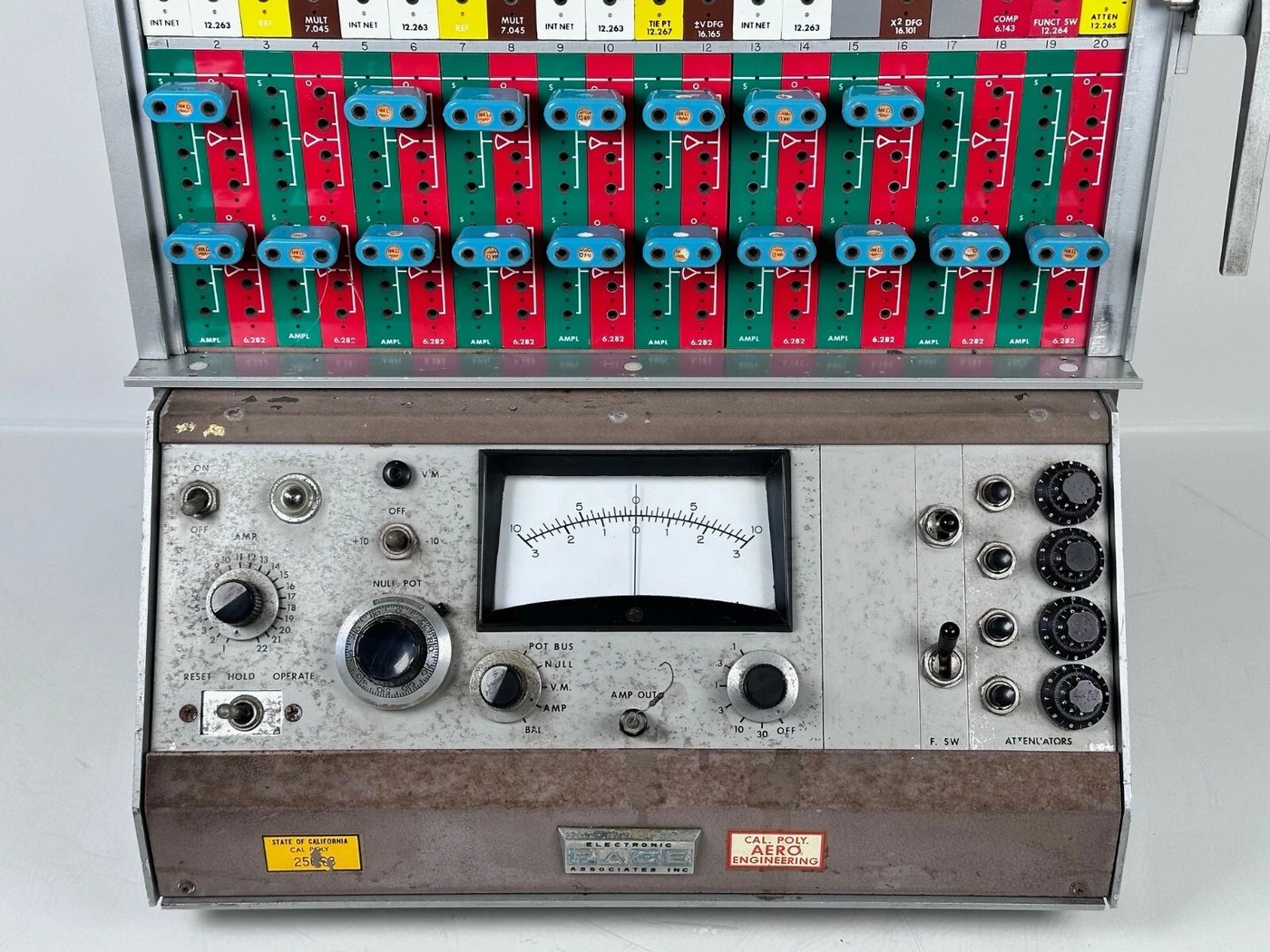
Figure 4 — The patch field at close range. Each vertical coloured strip is one module’s front face; the schematic symbol printed on it shows which holes are inputs, which are outputs, and how they relate. Photograph: locally held collector image of serial no. 70.

2.4.1 The Brochure’s Architecture

The brochure describes an arrangement in which there is no separate patch panel at all:

“All components plug into the computer console from the front of the computer… the computer patch panel is automatically formed by the color coded patching module forming the front of each component.”

Each module’s face is a patch panel section of standard height — 5 inches — and of ¾-inch or 1½-inch width matching the module behind it. Plugging the module in inserts its patch panel into the field. Removing it takes that section of the field away with it.

The consequence is that the machine’s programming surface reconfigures itself automatically when the complement changes, and that the printed symbol on each face documents the module immediately behind it. It cannot become out of date, because it is physically part of the thing it describes.

2.4.2 The Colour Code

Colour carries the function of each termination. The specification gives the scheme at §2.8 and again, with two additions, at §11.7.2:

Table 4 — Colour carries the function of each termination. The specification gives the scheme at §2.8 and again, with two additions, at §11.7.2

Colour	Meaning
Green	input
Red	output
Yellow	potentiometer
Black	ground
White	integrator networks
Tan	switching and non-linear components

In practice the brochure’s per-module colour assignments extend this and, in one respect, cut across it. The reference panel and the multiplier both use yellow for minus reference rather than for a potentiometer; the dual coefficient potentiometer uses brown for its control-knob area and yellow only for its patching area. The code should therefore be read as a strong convention rather than a strict grammar, and the printed symbol on the module face is the authority.

Table 5 — 4.2 The Colour Code

Module	Face colour(s) as stated in the brochure
Dual operational amplifier 6.282	green (inputs), red (outputs)
Dual integrator network 12.425	white
Dual coefficient pot 42.187 / 42.188	brown (control knob area), yellow (patching area)
Quad coefficient pot group 2.128	yellow
Multiplier 7.045	brown (inputs, outputs), black (ground), red (plus reference), yellow (minus reference)
Variable / log / X² DFG	brown
Comparator 6.143	green (inputs), red (relay contacts)
Dual function switch group 2.127	red (switch contacts), black (ground)
Reference panel 12.266	red (+ref), yellow (−ref), black (ground)
Dual tie point panel 12.267	white
Overload alarm 13.012	yellow

2.4.3 The Divergence

Specification §11.7 describes something else entirely. Under the heading Pre-Patch Panel it requires:

“The computing console shall accept a removable pre-patch panel. All computing components shall terminate inputs and outputs on this pre-patch panel. Construction shall be such as to eliminate possibility of ‘open’ connections due to loose or partial insertion of patch cords. The pre-patch panel shall be constructed so that it can be modified to conform to changes in the number and type of computing components in the computing console. This shall be accomplished by adding or replacing component blocks on the pre-patch panel as required by the new computer component configuration without any changes or additions to systems wiring. The pre-patch panel shall be at least 16-25/64 in width and 12-23/32 in height in order to allow the programmer proper access to, and vision of, the pre-patch panel connections.”

That is a conventional removable programming board of roughly 16⅜ by 12¾ inches, of the kind that lets one problem be patched up, lifted out and stored while another is run. It is not what the brochure describes and not what is visible in the photographs of either surviving console examined for this series, where the patch field is plainly the assembled module faces and is not removable.

Three readings are possible, and the held documents do not decide between them:

1. The specification describes a variant or option — a pre-patch-panel version of the TR-10 that the brochure does not cover.
2. The specification describes an earlier or later design stage that the shipped machine departed from.
3. The specification was drafted from a house template used for EAI’s larger consoles, where removable pre-patch panels were standard, and this clause was not reconciled with the TR-10’s actual construction.

The third is the most economical explanation, and the colour-code clause supports it: §11.7.2 restates the §2.8 colour list and adds white and tan — precisely the two colours the brochure assigns to module faces. But this is inference. What can be said without inference is that the TR-10 as photographed and as sold in the brochure has no removable pre-patch panel, and that a specification bearing EAI’s own letterhead requires one.

Note — This matters for anyone reading a TR-10 reference elsewhere. A source describing the machine as having a removable problem board is not necessarily wrong about some machine; it may be following PS 6305. It does not describe the consoles photographed here.

---

2.5 Power Distribution

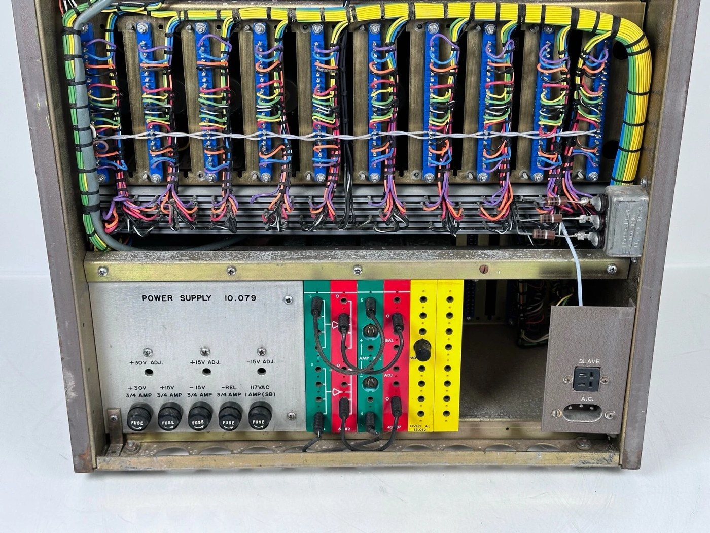
Figure 5 — The power supply, itself a plug-in unit, carrying the type number 10.079 on its face. The coloured terminal strips above it are the rear terminations of the bus-bar distribution. Photograph: locally held collector image of serial no. 70.

2.5.1 Bus Bars and Taper Pins

Specification §2.6 states the scheme and, in the same clause, its service rationale:

“All power supply voltages are to be supplied by bus bars. It shall be possible to remove any power supply voltage from any component by merely unplugging the proper taper pin from a bus bar carrying that voltage behind the component.”

This is the same architectural idea as the plug-in patch panel, applied to power: distribution is a shared structure that every module taps, and the tap is a single mechanical connection that can be broken without tools and without disturbing anything else. Isolating a suspect module for fault-finding is a matter of pulling one pin.

The brochure states the benefit in its own terms: “Bus bar power distribution eliminates complex cabling and simplifies maintenance.” Specification §2.7 adds that “all operational components and power supplies are to be of a plug-in type” — the supply is a module like any other, which is why it carries a type number of its own.

2.5.2 The Supply Itself

Table 6 — 5.2 The Supply Itself

Parameter	Value	Source
Type	transistorised	spec §10.1
Input range	100 to 125 V, 50 to 60 cycles per second	spec §10.1
Stated input on the brochure	115 V, 50–60 cycle	brochure p. 13
Input on the console data plate photographed	110 V, 50/60 cy, ½ A	data plate, serial no. 70
Capacity requirement	sufficient for the computer “when it is completely expanded”	spec §10.2
Consumption	under 50 W fully expanded (p. 13); “no more power than a 60 watt light bulb” (p. 2)	brochure, contradicting itself

The specification’s requirement is the useful one: accuracy must not vary across the whole 100–125 V input range. That is a stiffer constraint than a nominal figure, and it is the reason the supply is regulated rather than merely rectified.

2.5.3 Reference

The reference supply is separate from the power supply and is a computing element in its own right, because its voltage is the machine’s unity. Specification §9 requires “accurate ±10 volt reference supplies of 50 milliamperes capacity”, and that the patch panel carry “at least three parallel terminations for positive (+) reference and three for negative (−) reference”. Every coefficient potentiometer setting, every initial condition and every constant term in a problem is ultimately a fraction of this voltage; Vol 4 makes that dependence explicit.

---

2.6 The Control Panel

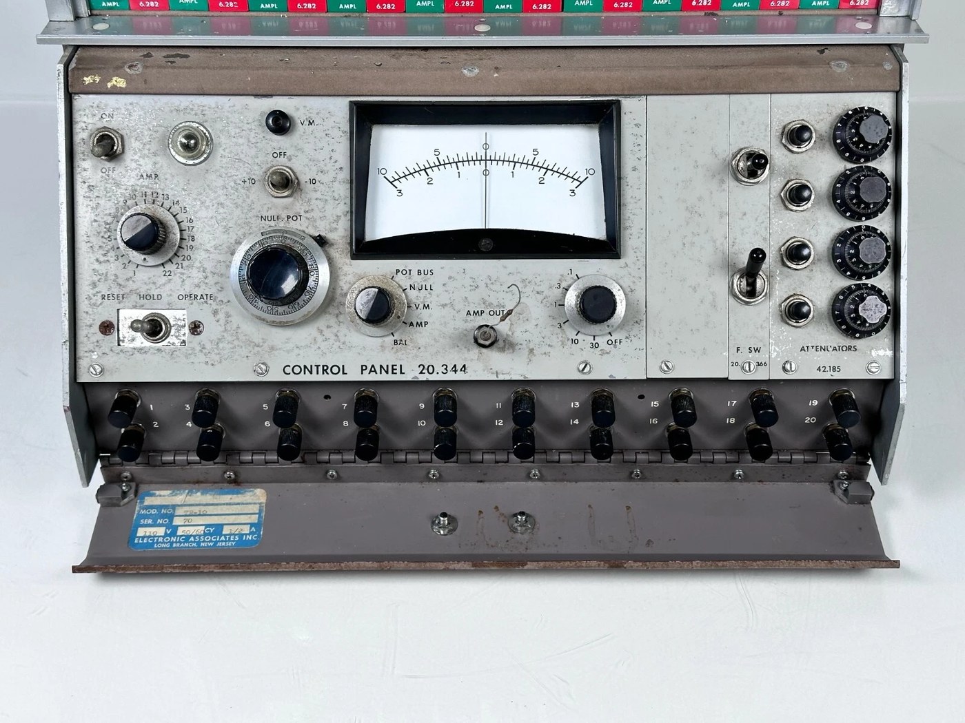
Figure 6 — The inclined control panel. The grid at far left is the individual overload indicator; the large dial below it selects an amplifier for readout; the null meter dominates the centre; the compute-time and repetitive-operation controls occupy the right, with the attenuator readout at the far right. Photograph: locally held collector image of serial no. 70, control panel type 20.244.

2.6.1 What It Is For

The specification’s §2.4 lists the control panel’s duties, and they divide cleanly into three: selecting the computer’s mode, reading a value without patching, and setting a coefficient without patching. The second and third are the interesting ones, because they are what distinguish a professional console from a teaching machine. On a machine without them, every measurement costs a patch cord and an interruption.

2.6.2 Mode Control

Three modes, specified at §2.4.1:

Table 7 — Three modes, specified at §2.4.1

Mode	Specified behaviour
RESET	”shall restore problem to initial conditions”
HOLD	”shall hold problem solution”
OPERATE	”shall place computer in operate condition”

The mode buttons drive relays located inside each integrator network rather than switching signals at the panel — see Vol 3 §3 and the note in Vol 5 on why that placement matters for repetitive operation.

2.6.3 Readout

The panel meter is a dual-purpose instrument. Specification §2.4.2.1 requires “a current sensitive meter… which may be used as a null meter with .1 % accuracy and as a voltmeter with 2 % accuracy”, with voltmeter ranges of ±30, ±10, ±3, ±1, ±0.3 and ±0.1 volts.

The accuracy asymmetry is the point. As a voltmeter it is a 2 % instrument, which is coarse against a machine whose amplifiers hold 20 µV offsets. As a null detector, where it only has to decide whether a difference is zero, it resolves to 0.1 %. Precise readings are therefore taken by nulling against a calibrated precision potentiometer — the NULL POT on the panel — and reading that potentiometer’s dial, not by reading the meter’s deflection. The meter’s job is to say “not yet”.

Three further requirements make the readout patchless:

• §2.4.2.3 — “It shall be possible through the use of no more than one patch cord to read any output voltage in the computer on the voltmeter and to null it against the null pot.”
• §2.4.2.4 — “It shall be possible to select and readout on the voltmeter the output of each operational amplifier (1 thru 20), plus (+) reference voltage, and minus (−) reference voltage without patching.”
• §2.4.2.5 — an amplifier output jack, so that selected amplifier outputs “are available at all times for metering, recording, etc.”

That second clause resolves something visible in the photographs. The amplifier selector dial and the overload indicator grid on the console both run to 22, not 20, on a machine that holds at most 20 amplifiers. Twenty amplifiers plus a positive-reference position plus a negative-reference position is exactly twenty-two. The two extra positions are the reference polarities, exactly as §2.4.2.4 requires.

2.6.4 Coefficient Setting and Balance

Specification §2.4.3 requires that “it shall be possible to accurately set any coefficient potentiometer within the system without patching”, and the brochure describes the mechanism: a push-button switch on each potentiometer module “connects reference to top of potentiometer and allows coefficient setting to be monitored by null meter”. The operator selects a pot, presses its button, and turns its ten-turn dial until the null meter nulls — reading 0.1 % without a single patch cord moved.

Amplifier balancing works the same way. Specification §2.4.4: “It shall be possible to select the stabilizer output of each operational amplifier and monitor it on the meter… to allow accurate balancing without patching.”

2.6.5 The Overload Alarm

Specification §2.5 requires “a visual overload alarm… which shall indicate whenever an operational amplifier is overloaded”, and §3.2 puts an overload indicator on each amplifier, “tied to a central overload alarm which will indicate any excessive departure of the summing point voltage from the zero.”

The brochure explains why this is worth a dedicated panel feature rather than an afterthought: “An important feature of the panel is the Individual Overload Indicator on the left side which immediately identifies any amplifier that is in an overload condition so that programming errors can be located with minimum delay.”

This is a diagnostic aimed squarely at the commonest failure mode in analog programming. An amplifier driven past ±10 V stops obeying the equation and the solution silently becomes meaningless — the machine goes on producing a smooth, plausible curve that is simply wrong. The indicator converts that silent failure into a visible one, and identifies which amplifier to rescale. Vol 4 §4 treats the scaling discipline that exists to prevent it.

An audible alarm was available as well: the Overload Alarm, Type 13.012, “provides an audible warning signal when an overload occurs in any of the operational amplifiers”, with an adjustable warning tone. It is part of the Standard Basic complement.

---

2.7 What the Architecture Buys, and What It Costs

What it buys. Capability becomes inventory. The console is a fixed asset that never changes; what the machine can do on any given day is decided by which modules are in the cupboard. Two organisations with the same console and different module stocks have materially different computers. Servicing follows the same logic: a suspect amplifier is swapped in under a minute and diagnosed later on the service shelf, while the problem carries on running.

What it costs. Three things, all visible in the rules above.

Geometry becomes a constraint on programming. Because a full-width module occupies a fixed odd-even pair, and because function generators may only sit in even positions, the physical layout of a problem is not free. A complement that is legal in aggregate can still be unplaceable.

The program is not portable. The patch field is the module faces, so a patched-up problem cannot be lifted out and stored — the very thing the specification’s pre-patch panel exists to allow. Re-running last month’s problem means patching it again from the information flow sheet. This is the practical cost of §4.3’s divergence, and it falls on the operator every time.

The machine’s documentation is distributed across its own hardware. The symbol on each module face is authoritative, which is excellent while the modules are present and unhelpful when a console arrives with empty positions — as surviving machines often do.

---

2.8 What Comes Next

Vol 3 takes the modules one at a time: what each contains, what it is specified to achieve, its type number and its patch-panel dimensions. Vol 4 lays a differential equation onto the hardware described here. Vol 5 returns to the integrator networks and the control panel’s compute-time control to treat time scaling and repetitive operation. Vol 6 prints specification GPAC-TR-10 PS 6305 clause by clause against the brochure, including the pre-patch-panel divergence set out in §4.3 above.