EAI PACE TR-10 — Volume 5 — Time scaling & repetitive operation

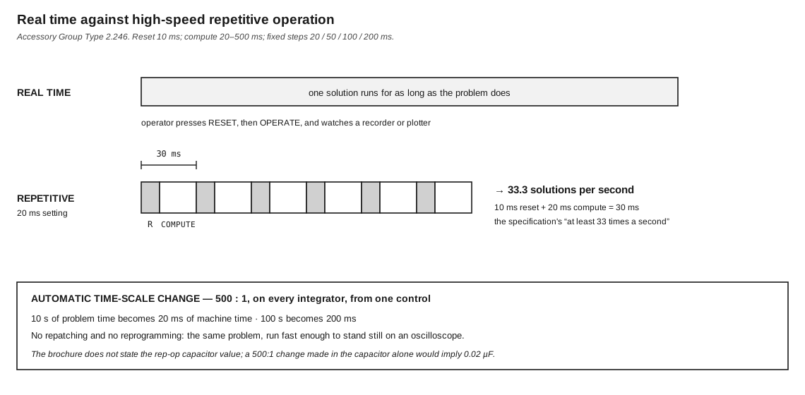
Figure 1 — Real time against high-speed repetitive operation. The 33-solutions-per-second figure in the specification is exactly 10 ms of reset plus 20 ms of compute. Diagram authored for this dive.

5.1 About this Volume

Volume 4 treated amplitude scaling — mapping a problem’s magnitudes onto ±10 V. This volume treats the other axis. An analog computer does not merely produce the right answer; it produces it at a particular speed, and that speed is a design variable the operator controls.

Three things are developed here: how the choice of integrator gain sets the relationship between problem time and machine time; how a uniform factor β applied to every integrator rescales that relationship without touching the solution; and what EAI’s High Speed Repetitive Operation accessory does to exploit it.

The specification’s own numbers for repetitive operation turn out to be internally consistent to the millisecond, and demonstrating that is a useful check on both the document and this reading of it. Where a figure is this series’ inference rather than EAI’s statement, it is marked as such.

Cross-references: Vol 3 §4 for the integrator networks; Vol 4 for amplitude scaling; Vol 6 for the specification clauses quoted here.

---

5.2 Integrator Gain Is the Machine’s Clock

5.2.1 The Basic Relation

An integrator built from an amplifier and an integrator network produces

        1
e₀ = − ---- ∫ e_i dt
       R_i C

The quantity 1/(R_i C) is the integrator gain, in units of inverse seconds. It is the only place in the machine where the units of time enter. Everything else — summers, potentiometers, multipliers, function generators — is instantaneous and dimensionless.

With the Type 12.425 network’s 10 µF capacitor and the four catalogued input resistors, the available gains are exact decades (Vol 3 §4.2):

Table 1 — With the Type 12.425 network's 10 µF capacitor and the four catalogued input resistors, the available gains are exact decades (Vol 3 §4.2)

Input resistor	R_i C	Gain
1 kΩ	10 ms	100 s⁻¹
10 kΩ	100 ms	10 s⁻¹
100 kΩ	1 s	1 s⁻¹
1 MΩ	10 s	0.1 s⁻¹

A gain of 1 s⁻¹ means that a constant input of 1 V produces an output ramping at 1 V per second. The machine’s second is the operator’s second: this is real time.

5.2.2 What Real Time Buys

Real-time operation is not merely the default; it is the reason analog machines survived as long as they did. A TR-10 running a control-loop problem in real time can be connected to real hardware — the simulated part and the physical part exchange voltages continuously, and the combination runs at the speed the physical part insists on. No digital machine of the period could do this for a general non-linear system.

It is also the mode in which a slow, accurate output device makes sense. The brochure’s external read-out equipment is an X-Y plotter (Model 1100E Variplotter) and a two-channel strip-chart recorder — instruments with pens and paper and mechanical time constants, entirely unsuited to anything faster than real time.

5.2.3 Where Real Time Fails

Two situations break it, from opposite ends.

The problem is too slow. A thermal process with a time constant of an hour, or a population model over decades, would take an hour or decades to run. Nobody waits.

The operator wants to iterate. The distinctive value of an analog computer is that a parameter can be changed by turning a knob and the effect seen at once. If each solution takes thirty seconds, a sweep of one parameter through ten values takes five minutes of watching. If each solution takes thirty milliseconds, the same sweep is continuous and the display appears to respond to the knob in real time. This is a qualitative change in how the machine is used, not merely a quantitative one.

Both are solved by the same mechanism.

---

5.3 The Time-Scale Factor β

5.3.1 The Derivation

Suppose every integrator gain in a program is multiplied by the same constant α. Write the machine’s own time as t_m.

Each integrator now computes ∫ over t_m with gain αg in place of gain g. Substituting t_p = α·t_m converts every such integral back into ∫ over t_p with gain g — which is the original program. The two are the same equation in different time variables.

Therefore: multiplying every integrator gain by α makes one unit of problem time elapse in 1/α units of machine time. The solution’s shape, its magnitudes, its initial conditions and every pot setting that is not an integrator input are all unchanged. Only the rate at which it is traced out changes.

This is the whole of time scaling. Two consequences follow immediately and both matter in practice:

1. The change must be uniform. Scaling some integrators and not others does not rescale time — it changes the problem, usually into a different and wrong one.
2. Initial conditions must not be scaled. They are values, not rates. An IC voltage is where a variable starts, and starting somewhere else is a different problem.

5.3.2 EAI’s Convention

The brochure’s Van der Pol program (Vol 4 §7) carries a factor written β, with the annotation “A time scale factor β is included in all the inputs to all the integrators to permit changes in the speed with which the solution is produced.”

On EAI’s diagram β appears as a divisor in the integrator-input pot settings — 1/(2β), λ/β, 2/β, 10λ/(4β) — so in their convention α = 1/β and increasing β slows the solution down. At the annotated β = 5.0 the program runs five times slower than its natural rate, which suits the phase-plane plot on an X-Y plotter that the example produces.

The internal evidence that this reading is right was set out in Vol 4 §7.4 and is worth restating, because it is the kind of check that catches a misreading: exactly the four integrator-input pots carry β, and neither of the two initial-condition pots does — precisely the division that §3.1 requires. The linear example of Vol 4 §4, which runs in real time and is plotted against seconds, carries no β at all.

Note — Conventions differ between manufacturers and textbooks on whether the time-scale factor multiplies or divides. The direction is a notational choice, not a fact about the hardware. What is invariant is that a uniform change to every integrator gain rescales time and nothing else. When reading any analog program, determine the direction from the pot settings rather than from the symbol.

5.3.3 Doing It With Resistors Instead

Because the gains available from the input resistors are exact decades, a factor of ten in time scale can be had without touching a single potentiometer: change every integrator’s input resistor from 100 kΩ to 10 kΩ and the program runs ten times faster, with every pot setting untouched.

This is the cheapest possible time-scale change, and it is limited to decades. Intermediate factors need the pot settings adjusted, which is what β does. The distinction matters when reading a surviving program sheet: a change of resistor type is a time-scale change that leaves no trace in the pot settings at all.

---

5.4 High Speed Repetitive Operation

5.4.1 The Accessory

Accessory Group Type 2.246 converts the TR-10 between real-time and high-speed repetitive operation. Its control panel occupies control-panel position CP1 (Vol 2 §2.1), and it is listed as optional on the Standard Non-Linear Expanded complement (Vol 3 §11.2).

The brochure’s summary of what it is for:

“In REPETITIVE OPERATION the computer is continuously recycled between the RESET and COMPUTE mode of operation. The problem is, therefore, solved over and over at some predetermined repetition rate, usually often enough to allow its presentation on an oscilloscope.”

5.4.2 The Specified Numbers

From specification §11.6 and the brochure’s page 5, which agree:

Table 2 — From specification §11.6 and the brochure's page 5, which agree

Parameter	Value
Compute time per solution	20 to 500 ms
Fixed switch-selected values	20, 50, 100, 200 ms
Vernier between fixed values	continuous, up to 2.5× the fixed value
Reset time	10 ms
Minimum cycling rate	at least 33 solutions per second
Automatic time-scale change	500 : 1 from real time to repetitive
Timing unit	completely solid state
Mode switching	high-speed electro-mechanical relays
Slave	control of two or more computers in either mode

5.4.3 The Numbers Close

Three independent consistency checks, all of which pass. This is worth doing because it is the strongest available evidence that these figures are engineering values rather than marketing ones.

The repetition rate. Reset takes 10 ms and the shortest compute time is 20 ms. One complete cycle is therefore 30 ms, giving

1 / 0.030 s = 33.33 solutions per second

which is exactly the specification’s “at least 33 times a second”. The figure is not a round number chosen for effect; it is the arithmetic consequence of the other two.

The vernier ceiling. The largest fixed compute time is 200 ms and the vernier extends to 2.5 times a fixed value:

200 ms × 2.5 = 500 ms

which is exactly the stated upper bound of the 20–500 ms range. The range’s top end and the vernier’s multiplier are the same fact stated twice.

The time-scale ratio against the compute times. At 500:1, the problem times corresponding to the four fixed settings are:

Table 3 — The time-scale ratio against the compute times. At 500:1, the problem times corresponding to the four fixed settings are

Compute time	Problem time at 500:1
20 ms	10 s
50 ms	25 s
100 ms	50 s
200 ms	100 s

A set of round problem intervals — 10, 25, 50 and 100 seconds — which is what one would choose if the switch positions were designed around the time-scale ratio rather than the other way round.

5.4.4 Why 500:1 and Not More

The ceiling is set by the amplifiers. Specification §3.4 requires a bandwidth of at least 200 kc, and §3.5 and §3.9 bound the phase shift and dynamic amplitude error at 1 kc. A solution compressed by 500 shifts every frequency in it up by 500. A problem whose interesting dynamics sit at a few hertz in real time lands at a few kilohertz when compressed — comfortably inside a 200 kc amplifier but already in the region where the specified dynamic errors are the ones being quoted. Compressing by 5000 instead would put the same dynamics at tens of kilohertz and the multiplier’s 0.28° phase shift at 1 kc would no longer be the relevant figure.

The brochure’s own claim is careful on exactly this point: the accessory “utilizes the wide bandwidth of the TR-10 Computing Components… with no loss in real time computing accuracy, changing the computer operation from real time to high speed repetitive operation is accomplished by a single control.” The claim is that real-time accuracy is not sacrificed by having the accessory fitted — not that accuracy in repetitive mode equals accuracy in real time.

5.4.5 The Comparator Floor

One component sets a hard limit that the brochure does not draw attention to. The comparator (Type 6.143) has a specified switching time of ≤ 10 ms (Vol 3 §8.1).

At the fastest repetition rate the entire compute interval is 20 ms. A comparator that takes up to 10 ms to change state consumes half of it. Any problem containing a discontinuity represented by a comparator — a limit stop, a switching control law, a contact — therefore cannot be run at the fastest settings without the discontinuity being smeared across a substantial fraction of the solution.

This is not a defect; it is the natural consequence of representing a decision with a relay. But it means the accessory’s speed range is fully available only to continuous problems, and an operator with a comparator in the patch should work at 100 or 200 ms.

---

5.5 What the Rep-Op Network Changes

5.5.1 Two Networks, One Function

The machine has two integrator networks (Vol 3 §4.3):

Table 4 — The machine has two integrator networks (Vol 3 §4.3)

Type	Role
12.263	real-time integrator network; shipped in both standard complements
12.425	repetitive-operation integrator network; part of the 2.246 accessory

The brochure is explicit that one replaces the other:

“This network replaces the real time, Type 12.263 Integrator Network in those TR-10 Computers equipped with the REP OP Accessory. Each REP OP Integrator Network contains the precision feedback capacitors, provisions for introducing initial conditions, and switching relays required to connect and operate two operational amplifiers as either real time or repetitive integrators. Patching interconnections are the same as those for the real time integrator networks.”

Three things follow. The rep-op network carries both sets of feedback capacitors, since it can serve as either kind of integrator. The switch between them is electrical, driven from the control panel, which is what makes the change “accomplished by a single control… without any reprogramming or repatching”. And because the patching is identical, a program written for a real-time machine transfers unchanged.

5.5.2 The Capacitor Value — An Inference

The brochure states the 500:1 ratio and gives the real-time capacitor as 10 µF ±0.1 % polystyrene. It does not state the repetitive capacitor’s value.

If the entire 500:1 change were made in the capacitor alone, with input resistors unchanged, the required value would be

10 µF / 500 = 0.02 µF

That is a practical polystyrene value and the brochure’s emphasis on “precision polystyrene feedback capacitors” for the accessory is consistent with it. But the ratio could equally be split between capacitance and resistance, or achieved with a value that is round in some other way.

Note — 0.02 µF is this series’ arithmetic, not EAI’s statement. It is recorded because it is the figure a restorer would need, and flagged because a document could contradict it. Vol 6 lists it among the items that would be settled by the TR-10 maintenance manual.

5.5.3 Where the Relays Live

The mode relays are inside the integrator networks, not on the control panel (Vol 3 §4.1). The panel’s RESET / HOLD / OPERATE buttons energise them; they do not themselves switch signals.

This is the architectural decision that makes everything in §6 possible, and it is worth appreciating as a decision. Putting the relays at the panel would have been simpler and would have worked identically for ordinary use. Putting them in the networks means each integrator’s mode is, physically, independently controllable — the wiring to make them act together is a choice made outside the module, not a constraint built into it.

---

5.6 Individual Mode Control: The 1965 Field Modification

5.6.1 What Was Missing

By 1965 EAI’s newer desk-top machines had a capability the TR-10 lacked. The company’s German dealer newsletter, EAI-Report No. 001 of July 1965, states the problem directly:

“The operating modes ‘Reset’ (initial conditions), ‘Hold’ (hold), and ‘Operate’ (compute) are normally controlled simultaneously for all integrators from a central switch. Control voltages switch the corresponding relays in all integrating networks. In many applications, particularly in automatically operating iterative procedures, individual control of the operating modes of individual integrators is essential. This capability is provided in the integrating networks of the analog computers TR-48 and TR-20.”

On the TR-48 and TR-20 the three control voltages are brought out to the patch panel, so that each integrator’s relays can be driven directly or through switching logic. On the TR-10 they were not.

5.6.2 Why It Matters

The applications the newsletter names — “automatically operating iterative procedures” — are the ones where the machine solves a problem repeatedly and uses the result of one solution to set up the next. Holding one integrator while others continue, or resetting part of a problem without resetting all of it, is what makes an iterative or boundary-value method possible. Without individual mode control, the machine can repeat a solution but cannot easily build on it.

5.6.3 The Modification

The newsletter gives a complete field procedure, and it is the most circuit-specific information about the TR-10 in any source held here:

“All integrating networks of the TR-10 with repetitive operation can be brought up to the latest standard by a small modification. Only the plastic patch panel of network L2.425 [12.425] is exchanged for a patch panel of the TR-20 integrator L2.1115 [12.1115], and the following connections are made (see TR-10 Maintenance Manual, sheet B 012 425 OS, Schematic Integrator Netw.).”

The connections:

Table 5 — The connections

Signal	Rear connector P1 contact	Routed via patch panel terminals
Reset	R	16 and 8
Operate	K	15 and 7
Time-Scale	E	14 and 6

And the procedure: “one simply removes the soldered bridges on the underside of the printed circuit for contacts R and K, and cuts the corresponding printed connection for contact E.”

The terminal correspondence between the two patch panels, as printed:

Table 6 — The terminal correspondence between the two patch panels, as printed

Type 12.425	Type 12.1115	Connection point on card
IC	IC	1 or 5
O	O	2 or 6
IN	SJ	3 or 7

5.6.4 What the Modification Reveals

Four things, none of them stated anywhere else in the held record.

There are three control voltages, not two. Reset (R), Operate (K), and Time-Scale (E). The newsletter explains the third: it “causes, in fast-repetitive operation, an automatically smaller time constant of the integrators.” That is the 500:1 change of §4.2 and §5.2, and this confirms it is commanded by a dedicated control line reaching every integrator network — consistent with the brochure’s “accomplished simultaneously on all integrators from mode control buttons on control panel”.

Hold is the absence of both. The newsletter: “for ‘Reset,’ for ‘Operate’ (the absence of both gives the ‘Hold’ position)”. Hold is not a signal; it is the state with neither relay energised — exactly the “both paths open” condition of Vol 3 §4.1.

Only rep-op machines qualify. “All integrating networks of the TR-10 with repetitive operation”. The modification applies to the 12.425 network, not the real-time 12.263, because only the former has a Time-Scale line worth bringing out.

The maintenance manual existed and was specific. “Sheet B 012 425 OS, Schematic Integrator Netw.” — a drawing number tying the sheet to the 12.425 network. That document would answer the capacitor question of §5.2 directly. It is not held here (Vol 1 §3.2).

Tip — A TR-10 encountered today whose integrator patch panels carry terminals numbered to 16 has had this modification, or was built after it became standard. The patch panel is the visible evidence, since the modification is precisely a patch-panel exchange.

---

5.7 Reconciling the Museum’s Fifteen to Sixty Seconds

Volume 1 §4 recorded the National Cryptologic Museum’s exhibit placard, which states that “the ideal duration of a single run was from 15 to 60 seconds, not counting set-up time.”

That figure cannot be a property of the machine as EAI describes it. In real time a solution runs for as long as the problem requires — there is no 15-second floor and no 60-second ceiling. In repetitive operation a solution takes 20 to 500 milliseconds, two to three orders of magnitude away.

The reconciliation is straightforward once the modes are separated. The placard is describing how that installation used the machine: a real-time run, plotted on a recorder, of a length chosen to be long enough to show the transient and short enough not to accumulate integrator drift. Fifteen to sixty seconds is a thoroughly sensible working range for exactly that, and it sits comfortably inside the 10-to-100-second problem intervals that §4.3 showed the repetitive settings were designed around.

Read as operational practice the placard is unremarkable and probably accurate. Read as a specification it is simply a category error — and it is the kind of secondary claim that propagates into later accounts of a machine as though it were a rating.

---

5.8 Summary Table

Table 7 — Summary Table

Question	Answer	Source
What sets machine time?	integrator gain 1/(R_i C)	derived, Vol 3 §4.2
Real-time gain?	1 s⁻¹ with 100 kΩ and 10 µF	brochure + resistor catalogue
How is time rescaled?	uniform factor on every integrator input	derived, §3.1
Which pots carry it?	integrator inputs only, never initial conditions	brochure diagram, §3.2
EAI’s β direction	divisor: larger β is slower	brochure diagram, §3.2
Repetitive compute time	20–500 ms; fixed 20/50/100/200 ms	spec §11.6.2–3
Reset time	10 ms	spec §11.6.2
Cycling rate	≥ 33 per second (= 1/30 ms)	spec §11.6.2, checked §4.3
Time-scale change	500:1, all integrators, one control	spec §11.6.6
Rep-op network	Type 12.425, replaces 12.263	brochure p. 7
Rep-op capacitor	not stated; 0.02 µF by inference	§5.2
Control lines	Reset (R), Operate (K), Time-Scale (E)	EAI-Report No. 1, 1965
Fastest usable with a comparator	100–200 ms, not 20 ms	derived from spec §7.5, §4.5

---

5.9 What Comes Next

Vol 6 prints specification GPAC-TR-10 PS 6305 clause by clause against the brochure, collects every divergence noted across Volumes 2 to 5, and lists what would need to be found to settle the open questions — the maintenance manual above all. Vol 7 turns from the machine to its use: who operated it, what for, where it sat in EAI’s product line, and how the approach it represents was displaced.