EAI PACE TR-10 — Volume 4 — Programming & scaling

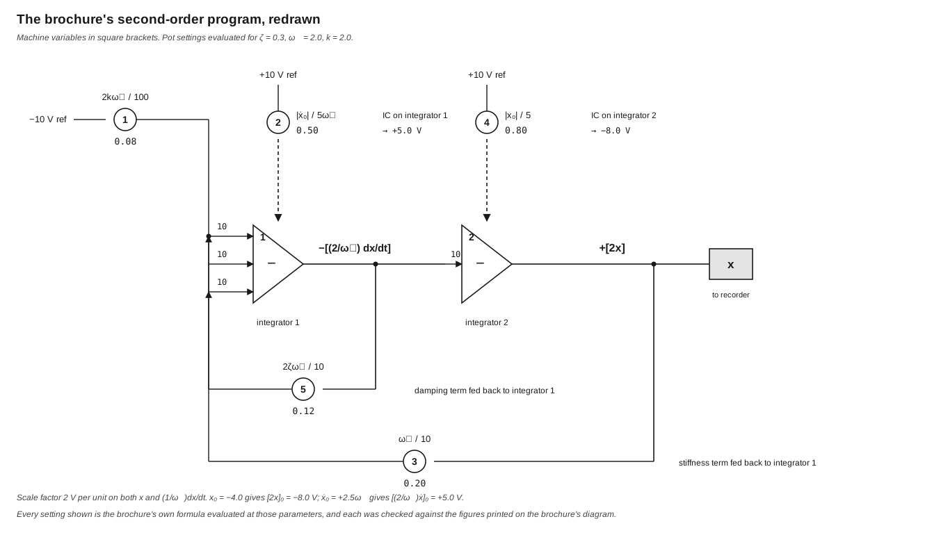
Figure 1 — The brochure’s second-order program, redrawn with the potentiometer settings evaluated for ζ = 0.3, ωₙ = 2.0, k = 2.0. Every setting shown was checked against the formula printed on EAI’s own diagram. Diagram authored for this dive.

4.1 About this Volume

This volume turns a differential equation into a patched machine. It covers the standard method of analog programming, develops amplitude scaling from first principles, and then works EAI’s own two published TR-10 programs — a linear second-order equation and Van der Pol’s non-linear oscillator — checking the arithmetic at every step against the figures printed in the brochure.

Scaling is where analog-computing writing most often goes wrong, so the approach here is to derive rather than assert, and to show the numbers. Where a step is this series’ own working rather than EAI’s, it is marked.

Time scaling is deliberately held back to Vol 5. This volume treats problems that run in real time; the machinery for making them run five hundred times faster is a separate subject and a separate accessory.

Cross-references: Vol 3 for the modules used here; Vol 5 for time scaling; Vol 2 §6.5 for the overload alarm that catches the errors this volume exists to prevent.

---

4.2 The Method

4.2.1 What the Machine Can Do

The TR-10 offers, in hardware: summation, multiplication by a constant between 0 and 1 (the coefficient potentiometer), multiplication by a decade gain (the choice of input resistor), integration with respect to time, sign inversion (unavoidably, since every amplifier inverts), multiplication of two variables (the 7.045), and arbitrary functions of one variable (the diode function generators).

It cannot differentiate — or rather, it can, but nobody does. Differentiation amplifies noise in proportion to frequency, and a differentiator built from the same parts as an integrator is unstable and useless. This single fact dictates the entire method that follows.

4.2.2 Integrate Down, Never Differentiate

Because integration is available and differentiation is not, every analog program is built by assuming the highest derivative exists, and integrating downwards to obtain the lower ones.

Consider any second-order equation. Rearrange it so the highest derivative stands alone on the left:

ẍ = (everything else)

Now suppose a voltage representing ẍ existed. Feeding it to an integrator yields ẋ; feeding that to a second integrator yields x. Both are now available. If the right-hand side can be assembled from x, ẋ, constants and the machine’s other operations, the loop closes: the output of the assembly is ẍ, which is what was assumed at the start. The circuit is consistent, and from the moment it is released from RESET its voltages are forced to satisfy the equation.

The brochure states the same procedure in three steps:

“1) Integrating the highest derivative of eq.4 twice to produce 2/ωₙ dx/dt and 2x. 2) Instrumenting the R.H.S. of eq.4 to complete the loops. 3) Providing a time-base generator by integrating a constant voltage in integrator 4.”

Note step 3. A plot against time needs a voltage proportional to time, and the machine makes one the same way it makes everything else — by integrating a constant. A fourth amplifier earns its keep producing nothing but a ramp for the recorder’s X axis.

4.2.3 Counting the Sign Inversions

Every TR-10 amplifier inverts. A summer produces −(g₁e₁ + g₂e₂); an integrator produces −g∫e dt. This is not a nuisance to be corrected everywhere; it is a resource to be counted.

A two-integrator loop inverts twice and therefore returns to the original sign, which is exactly what a negative feedback term requires. In the program of §4 below, the output of integrator 1 is −[(2/ωₙ)dx/dt] and the output of integrator 2 is +[2x] — the second inversion has restored the sign. A term that needs the opposite polarity from what the chain delivers costs one extra amplifier used as a plain inverter, and a well-planned program spends as few of those as possible.

Tip — The reliable discipline is to write the sign of every machine variable on the diagram beside the amplifier that produces it, as EAI does, before patching anything. A polarity error does not announce itself: it produces a smooth, plausible, wrong curve, or a prompt overload.

---

4.3 Amplitude Scaling

4.3.1 Why It Is Compulsory

A problem variable might be a displacement in metres, a temperature in kelvin, or a population in millions. The machine has one currency: volts, and only between −10 and +10 of them. Scaling is the translation, and it is not optional. Too small a scale factor wastes resolution and buries the answer in drift and noise; too large a one drives an amplifier into overload, at which point it stops obeying the equation and the solution becomes fiction.

The ±10 V limit is hard. Specification §3.3 gives the amplifier output as ±10 V at 20 mA, and the individual overload indicator (Vol 2 §6.5) exists precisely because exceeding it is both easy and silent.

4.3.2 The Scale Factor

The brochure’s definition, stated twice in its two worked examples:

                max allowable voltage
scale factor = ------------------------     (volts per unit)
                max value of variable

and then

scale factor × variable = scaled voltage

The scaled voltage is the machine variable, and EAI writes it in square brackets. If x is estimated never to exceed 5 units, the scale factor is 10/5 = 2 V per unit, and the machine variable is written [2x] — literally “the voltage that is two times x”.

This notation is worth adopting wholesale, because it makes the bookkeeping self-checking. Every quantity on the diagram carries its own scale factor in its name. An equation written entirely in square-bracket variables is an equation about voltages, and it can be read straight onto the hardware.

4.3.3 Choosing the Estimate

The weak link is “max value of variable”. It is an estimate, made before the problem has been solved — which is the reason the problem is being put on a computer in the first place. Three approaches, in the order an experienced operator would try them:

1. Analytic bound. For a linear system a steady-state value and a worst-case overshoot can often be written down. This is the safest and is what the brochure’s examples do implicitly.
2. Physical reasoning. A pendulum will not exceed its release angle; a tank will not exceed its capacity.
3. Run it and look. Scale conservatively, run the problem, observe the actual maxima, and rescale to use the full range. The TR-10’s repetitive mode (Vol 5) makes this cheap — the operator can watch the solution on an oscilloscope while turning the scale factor’s potentiometer.

Note — An over-conservative first pass costs resolution, not correctness. An over-optimistic one costs correctness. The asymmetry argues for guessing high on the maxima and rescaling once the behaviour is known.

4.3.4 Scaling the Derivatives Separately

A frequent error is to scale x and then assume ẋ inherits the same factor. It does not. Displacement and velocity are different physical quantities with different magnitudes, and each gets its own scale factor chosen from its own expected maximum.

In the brochure’s linear example both variables happen to receive the same factor of 2, but they are chosen independently and the equality is a coincidence of the numbers:

Table 1 — In the brochure's linear example both variables happen to receive the same factor of 2, but they are chosen independently and the equality is a coincidence of the numbers

Variable	Estimated maximum	Scale factor	Machine variable
x	5	2	[2x]
(1/ωₙ)(dx/dt)	5	2	[(2/ωₙ)dx/dt]

Note also which quantity was scaled: not ẋ but (1/ωₙ)ẋ. Dividing the velocity by the natural frequency before scaling makes the two variables comparable in magnitude for any ωₙ, so that one set of pot settings works across the parameter sweep ωₙ = 1, 2, 3. This is a deliberate and rather elegant piece of problem preparation, and it is easy to miss.

---

4.4 The Linear Second-Order Program, Derived

4.4.1 The Problem as Posed

The brochure sets the standard second-order system:

  1   d²x      2ζ   dx
 --- ----- + ---- ---- + x = k(t)                              (1)
 ωₙ²  dt²     ωₙ   dt

with initial conditions at t = 0

dx/dt = ẋ₀ = +2.5 ωₙ          x = x₀ = −4.0

and parameters ζ = 0.3, 0.6, 1.2; ωₙ = 1.0, 2.0, 3.0; k = 2.0, a constant.

4.4.2 Into Highest-Derivative Form

Multiply (1) through by ωₙ and isolate the highest derivative:

 1   d²x                    dx
--- ----- = kωₙ − 2ζωₙ (1/ωₙ ----) − ωₙ x                      (2)
ωₙ   dt²                     dt

This is the brochure’s equation 2, and it reproduces exactly. Note that the left-hand side is (1/ωₙ)ẍ rather than ẍ — the same normalisation by ωₙ that was applied to the velocity, carried through consistently.

4.4.3 Into Machine Variables

Multiply (2) by the scale factor 2:

 2   d²x                       2   dx
--- ----- = 2kωₙ − 2ζωₙ [--- ----] − ωₙ [2x]                   (3)
ωₙ   dt²                      ωₙ   dt

Every quantity in (3) is now a voltage. This is the brochure’s equation 3, and it too reproduces exactly.

4.4.4 Into Gains and Pot Settings

The final step splits each coefficient into an integrator input gain (a decade, set by the choice of input resistor — Vol 3 §4.2) and a potentiometer setting (a number between 0 and 1). The brochure’s equation 4:

 2   d²x        2kωₙ              2ζωₙ    2   dx          ωₙ
[--- -----] = 10(------)[10] − 10(-----)[--- ----] − 10(-----)[2x]   (4)
 ωₙ   dt²        10·10              10    ωₙ   dt          10

The brochure explains its own notation, and the explanation is worth quoting because it is the clearest statement of the convention in any of the sources:

“In this equation the terms inside the square brackets represent voltage outputs from the computer components, such as the output of an amplifier or from the reference source. The terms inside the parenthesis represent pot settings, and the factors without parenthesis or brackets indicate the required input gain to the first integrator.”

So each term is (input gain) × (pot setting) × (machine voltage), and the three are read off the diagram as the number beside the input arrow, the number in the circle, and the labelled signal.

4.4.5 The Numbers

Evaluating (4) at ζ = 0.3, ωₙ = 2.0, k = 2.0:

Table 2 — Evaluating (4) at ζ = 0.3, ωₙ = 2.0, k = 2.0

Term	Formula	Value	Integrator input gain	Product
Forcing	2kωₙ/100	2(2)(2)/100 = 0.08	10	0.8, applied to the 10 V reference → 8 = 2kωₙ ✓
Damping	2ζωₙ/10	2(0.3)(2)/10 = 0.12	10	1.2 = 2ζωₙ ✓
Stiffness	ωₙ/10	2.0/10 = 0.20	10	2.0 = ωₙ ✓

All three close against equation (3). Each pot setting lies comfortably inside the potentiometer’s 0-to-1 range, which is the practical test that the gain/pot split was chosen sensibly — a “required” setting above 1 means the input gain was chosen a decade too low.

4.4.6 The Initial Conditions

The two initial conditions of a second-order problem are exactly the two integrator IC voltages. Both are fractions of the +10 V reference, set on a coefficient potentiometer.

Table 3 — 4.6 The Initial Conditions

Condition	Problem value	Machine variable	Required voltage	Pot formula	Setting
x₀	−4.0	[2x]₀ = 2(−4.0)	−8.0 V	|x₀|/5	4/5 = 0.80
ẋ₀	+2.5ωₙ	[(2/ωₙ)ẋ]₀ = (2/ωₙ)(2.5ωₙ)	+5.0 V	|ẋ₀|/5ωₙ	2.5ωₙ/5ωₙ = 0.50

Both formulas are EAI’s, taken from the pots labelled ② and ④ on the printed diagram, and both evaluate to settings that produce the required voltages from a 10 V reference. The velocity condition is independent of ωₙ — the ωₙ cancels — which is again the normalisation of §3.4 earning its keep across the parameter sweep.

4.4.7 A Remark on Headroom

The scale factor of 2 was chosen from an estimated maximum of 5 for x. The brochure’s own solution plot, for ζ = 0.3, shows x peaking at very close to +5.

That means the machine variable [2x] reaches +10.0 V at the peak — the full output rating, with no margin whatsoever. Any slightly larger overshoot, any pot set a little high, or any amplifier a little out of balance would put that amplifier into overload at the most interesting moment of the solution.

This is an observation about EAI’s example, not a criticism of the method; a sales brochure demonstrating dynamic range has every reason to fill it. But it is a poor model for working practice. Scaling to about 80 % of full scale — a factor of 1.6 here rather than 2 — would cost 2 dB of resolution and remove the risk entirely. The overload indicator exists for exactly this situation, and on this program it would be worth watching.

---

4.5 The Gain-and-Pot Product

A short section, because one rule prevents most programming arithmetic errors.

Any coefficient c required by a scaled equation is realised as

c = (integrator or summer input gain) × (pot setting)

where the gain is one of 0.1, 1, 10, 100 (Vol 3 §4.2, §10.2) and the pot setting lies in [0, 1). Therefore:

Table 4 — where the gain is one of 0.1, 1, 10, 100 (Vol 3 §4.2, §10.2) and the pot setting lies in [0, 1). Therefore

Required coefficient	Gain to use	Pot setting
0.08	10	0.008 — too fine to set accurately
0.08	1	0.080
0.8	1	0.800
1.2	10	0.120
8.0	10	0.800
12	100	0.120

Choose the gain that puts the pot setting in the upper half of its range. A potentiometer set to 0.008 is using 8 turns out of 1000 and its 0.025 % resolution has become 0.3 % of the value being set; the same coefficient realised as gain 1 × 0.08 is ten times better, and as gain 0.1 × 0.8 better still. This is the analog equivalent of avoiding catastrophic cancellation, and it is free.

Note that the brochure’s forcing term does the opposite: 10 × 0.08. That is because the term’s pot also has to divide the 10 V reference by ten to produce a unity-valued constant, which absorbs one decade. The rule is a default, not a law.

---

4.6 The Van der Pol Program

4.6.1 Why This Example Matters

The second problem in the brochure is Van der Pol’s equation — the canonical non-linear oscillator, with a limit cycle that no linear analysis produces. It is the example that justifies the non-linear row, and it exercises the multiplier and the X² function generator together.

d²x           dx
--- − λ(1−x²) -- + x = 0                                       (1)
dt²           dt

for −5 < ẋ₀ < +5, −5 < x₀ < +5, and 0.1 < λ ≤ 2. The output wanted is a phase-plane plot — ẋ against x — rather than a time history.

4.6.2 Scaling

Table 5 — 7.2 Scaling

Variable	Estimated maximum	Scale factor	Machine variable
x	5	2	[2x]
dx/dt	10	1	[dx/dt]

Here the two factors genuinely differ, which makes this the better illustration of §3.4: the velocity is expected to range twice as far as the displacement, so it gets half the scale factor.

Solving for the highest derivative:

d²x     dx        dx
--- = λ -- − λx² -- − x                                        (2)
dt²     dt        dt

4.6.3 The Non-Linear Term

This is the step worth doing slowly, because it is where the factors of ten come from.

The term to be produced is λx²ẋ. In machine variables, x = [2x]/2, so

λ x² ẋ = λ ([2x]/2)² [dx/dt] = (λ/4) [2x]² [dx/dt]

But the machine cannot produce [2x]²[dx/dt] directly. It produces the chain:

1. The X² DFG (16.101) takes [2x] and yields [2x]²/10 — it divides by ten (Vol 3 §7.2).
2. The multiplier (7.045) takes that and [dx/dt] and yields ([2x]²/10)·[dx/dt]/10 = [2x]²[dx/dt]/100 — it divides by ten again (Vol 3 §6.1).

So the quantity actually available at the multiplier output is [2x]²[dx/dt]/100. To recover (λ/4)[2x]²[dx/dt] from it requires a coefficient of

(λ/4) × 100 = 100λ/4

which is exactly the coefficient the brochure prints in its equation 3:

d²x       dx     100λ  [2x]²  dx     1
[---] = λ[--] − (----)(-----)[--] − - [2x]                     (3)
 dt²      dt       4     10    dt    2

The brochure’s own comment — “Factors of 10 are included in the nonlinear term for they are produced automatically in the computer voltage representing this term” — is correct but terse. The factor of 100 is two successive divisions by ten, one from each non-linear component, and the factor of 4 is the square of the displacement’s scale factor. Both must be tracked or the limit cycle comes out the wrong size.

The linear terms check trivially: λẋ scales with factor 1 and is unchanged; x = [2x]/2 gives the −½[2x] term. Both appear in equation 3 as printed.

4.6.4 The Settings, With the Time-Scale Factor

The Van der Pol diagram carries a time-scale factor β, applied to every integrator input. Vol 5 treats what β does; what matters here is that it appears as a divisor in every integrator-input pot setting and is absent from the two initial-condition pots. The brochure’s diagram is annotated β = 5.0, λ = 2.0. Evaluating:

Table 6 — The Van der Pol diagram carries a time-scale factor β, applied to every integrator input. Vol 5 treats what β does; what matters here is that it appears as a divisor in every integrator-input pot setting and is absent from the two initial-condition pots. The brochure's diagram is annotated β = 5.0, λ = 2.0. Evaluating

Pot	Formula printed	At β = 5.0, λ = 2.0	Setting printed	✓
①	1/(2β)	1/10 = 0.1	0.1	✓
③	λ/β	2/5 = 0.4	0.4	✓
⑤	2/β	2/5 = 0.4	0.4	✓
⑥	10λ/(4β)	20/20 = 1.0	1.0	✓
②	|ẋ₀|/10	(no β — an initial condition)	—	—
④	|x₀|/5	(no β — an initial condition)	—	—

All four integrator-input settings reproduce. The pattern of which pots carry β and which do not is itself a check on the reading: exactly the four pots feeding integrator inputs carry the time-scale factor, and neither initial-condition pot does. Initial conditions are values, not rates, and rescaling time must not disturb them. Vol 5 §3 develops this.

Pot ⑥ at 1.0 is also worth noting: it is at the top of its range, which means the non-linear term is as large as the machine can make it at λ = 2. Running λ any higher would require a gain change, not merely a knob.

---

4.7 Before Pressing OPERATE

A checklist, assembled from the requirements the machine’s own design implies rather than from any single source.

Table 7 — Before Pressing OPERATE

#	Check	Why
1	Balance every amplifier in use	20 µV offset is the specification; an unbalanced amplifier integrates its own offset and the solution drifts (Vol 2 §6.4)
2	Verify the reference at ±10 V	every pot setting and every initial condition is a fraction of it (Vol 3 §9.1)
3	Set every coefficient pot against the null meter	0.1 % by null, not 2 % by meter deflection (Vol 2 §6.3)
4	Confirm each integrator’s input gain — the resistor, not the pot	a decade error here is the commonest large error
5	Trace polarity through the whole loop	every amplifier inverts; count them (§2.3)
6	Set initial conditions and check them in RESET	in RESET the integrator outputs are the ICs, so they can be read directly
7	Press OPERATE and watch the overload indicator, not the recorder	an overload invalidates everything downstream of it (Vol 2 §6.5)
8	Re-run with one parameter changed	a solution that does not respond sensibly to a known parameter is a patching error, not a discovery

Step 6 deserves emphasis because it is a free check that the machine offers and a digital simulation does not: in RESET, every integrator is holding its initial condition, so the operator can select each amplifier in turn on the panel and read back the ICs actually applied, before any computation happens.

---

4.8 Where Programs Go Wrong

Table 8 — Where Programs Go Wrong

Symptom	Likely cause	Where to look
Immediate overload on OPERATE	scale factor too large, or a sign error making feedback positive	§3.2, §2.3
Solution drifts steadily off with no input	amplifier out of balance, or an integrator with an unintended input	Vol 2 §6.4
Correct shape, wrong magnitude	an input-gain decade error, or a scale factor not divided back out when reading	§5
Correct magnitude, wrong shape	a coefficient set on the wrong pot, or a term patched to the wrong integrator	§4.5
Oscillation that should not be there	positive feedback from a miscounted inversion	§2.3
Limit cycle the wrong size (non-linear problems)	a missing factor of 10 from the multiplier or DFG	§7.3
Answer changes when the recorder is connected	loading; the amplifier is rated 20 mA and a low-impedance load matters	Vol 3 §3.1

Tip — The single most valuable habit is to solve one trivially checkable case first. Set ζ high enough that the system is overdamped and the answer is a known exponential, or set the non-linear coefficient to zero and confirm the linear behaviour. A program that gets the easy case right is very rarely wrong about the hard one in a way that scaling caused.

---

4.9 What Comes Next

Vol 5 adds the time axis: how integrator gains set the machine’s clock, what the time-scale factor β does, and how Accessory Group 2.246 compresses a hundred seconds of problem into two hundred milliseconds so that a solution can be watched on an oscilloscope. Vol 6 sets every specification figure used here against its source. Vol 7 places the machine and its method in the wider history.