Aeon Dynamic Simulator — Volume 6 — Operating the machine

The three-position lever, the initial-condition asymmetry as it bites in practice, the two readout instruments and what each is worth, the overload lamps, and a calibration sequence reconstructed from the test points

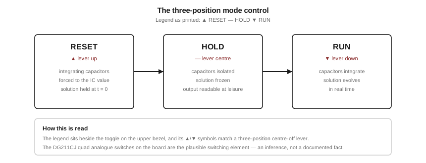
Diagram of the three-position mode control showing RESET, HOLD and RUN with the lever position and capacitor state for each.

Figure 1 — The three modes. Diagram authored for this dive from the panel legend; see photo_credits.txt.

6.1 About this Volume

This volume covers running the machine: what the mode lever does, how initial conditions are applied and what the asymmetry of Vol 3 costs in practice, how a result is read, what the indicator lamps are for, and how the machine would be calibrated.

The last of those requires a warning. No calibration procedure for this machine is held. The sequence set out below is a reconstruction — an account of what would have to be done, derived from the test points and adjustments visible in the photographs and from standard analogue-computer practice. It is not a manufacturer’s procedure, it has not been performed on a working machine, and it is presented as a framework for someone who has one, not as an authority.

Cross-references: Vol 2 for the bezel instruments; Vol 3 for the elements and the IC asymmetry; Vol 4 for the hardware and the test points; Vol 5 for the arithmetic.

6.2 The Three Modes

The machine’s entire operating control is one three-position toggle on the upper bezel, whose legend is printed on the patch overlay beneath it as ▲RESET — HOLD ▼RUN.

Table 1 — The Three Modes

Mode	Lever	What it does
RESET	up	Integrating capacitors are forced to their initial-condition values; the solution stands at t = 0
HOLD	centre	Capacitors are isolated; the solution is frozen wherever it had reached
RUN	down	Capacitors integrate; the solution evolves in real time

These are the three standard modes of an analogue computer and the legend states them plainly. What the legend does not state is how they are implemented, and Vol 4’s identification of two DG211CJ quad analogue switches on the computing board is the basis for the reading that mode switching is done electronically, by CMOS analogue switches steering each integrating capacitor, rather than by relay contacts. That is an inference from device type and quantity, not a traced circuit.

6.2.1 Why HOLD Matters

RESET and RUN are self-explanatory; HOLD is the mode that repays explanation, because it is what makes a slow instrument usable.

Freezing the solution mid-run allows the operator to read a value carefully from a meter that needs time to settle, to write down an intermediate result, or to inspect several points in a problem one after another with a single patch cord. On a machine whose only unaided readout is a 1.5 per cent needle instrument (Vol 2), the ability to stop time and read at leisure is not a luxury.

HOLD is also the machine’s own drift test, and the only one available. With the machine in HOLD and nothing patched to an integrator’s input, its output should stay where it is. The rate at which it instead creeps is the integrator’s drift, and it sets the longest useful HOLD. As Vol 5 records, no drift figure for this machine is held; this measurement is the only way to obtain one.

6.2.2 What Is Absent

There is no repetitive mode. The legend names three positions and no more: no rate control, no repetitive-operation setting, no run timer. A solution is started by hand, runs once, and is stopped by hand.

This is a real difference from the teaching machines of the previous generation. The Heathkit EC-1 offered a repetitive mode driven by a multivibrator precisely so that a solution could be re-run many times per second and stand still on an oscilloscope screen. The Aeon does not, and the most economical explanation is that the interface column (Vol 2) was expected to take over that duty: a host computer captures the single run and plots it, which is the more flexible arrangement and needs no rate control on the machine itself. This is a reading of an absence together with a presence, and it is marked as inference.

6.3 Initial Conditions in Practice

6.3.1 How an Initial Condition Is Set

Integrators 1 and 2 each carry a jack labelled IC with an arrow running into the amplifier. The conventional arrangement, and the one the panel’s symbol depicts, is that during RESET the integrating capacitor is charged to whatever voltage is presented at that jack, and that at the transition to RUN the capacitor is released and integration begins from there.

Setting a value is therefore a patching operation like any other: a coefficient potentiometer is patched across a reference strip, its wiper is taken to the IC jack, and its ten-turn dial sets the starting value as a fraction of 10 V. Both sign and magnitude are available, because Vol 3 established that the pots are ungrounded at both track ends and can therefore be patched from +10 to −10.

Note the cost: an initial condition consumes a potentiometer. A second-order problem needing two initial conditions and two coefficients uses four of the machine’s six pots.

6.3.2 The Asymmetry, and What It Forbids

Integrators 3, 4, 5 and 6 have no IC jack. On RESET their capacitors are necessarily driven to whatever the hardware drives them to with no external value presented — which for a capacitor shorted or forced to the reset node is zero.

The practical rule is therefore blunt: a problem may have at most two non-zero initial conditions, and they must be assigned to integrators 1 and 2.

This shapes how a problem is set up on this machine in three ways.

Assign the IC-bearing integrators first. Before patching anything, identify which state variables start at non-zero values, and place those on integrators 1 and 2. Everything else can go anywhere. A programmer who patches in the order the equations happen to be written will frequently find the non-zero initial condition stranded on integrator 5.

Re-order the problem if necessary. A system of equations can usually be renumbered so that the variables carrying non-zero starting values occupy the first two integrators. This costs nothing but attention.

Use a forcing input instead where possible. A non-zero initial condition and a step input applied at t = 0 are not the same thing, but for many teaching problems either will demonstrate the behaviour of interest. A step applied through an input resistor needs no IC jack, and can therefore be applied to any of the six integrators.

Where none of these work — a problem genuinely requiring three or more independent non-zero starting values — the machine as drawn cannot set it up. Vol 3 leaves open whether the missing IC inputs reflect a deliberate economy or circuitry not brought to the panel; either way the panel is what the operator has.

6.4 Reading the Answer

The machine offers three routes to a result, of very different quality.

6.4.1 The Analogue Meter

The centre-zero meter reads ±10 V directly, without a range switch, and its dial states an accuracy class of 1·5 — 1.5 per cent of full scale, or about ±0·15 V anywhere on the scale (Vol 2).

Set against a machine whose full range is ±10 V, that is roughly one part in seventy. It is entirely adequate for the meter’s real job, which is to show the shape of a solution as it evolves: whether an oscillation is growing or decaying, whether a system settles, roughly how long it takes, roughly what it settles to. It is not adequate for taking a three-figure answer off the needle, and no amount of care in reading it will make it so.

The METER 1 and METER 2 jacks in the interface column are the patchable inputs by which any point in a problem can be brought to a readout without disturbing the patch — two of them, so that two points can be left connected and compared.

6.4.2 The Digital Display

The LCD panel meter on the bezel is unlit in every held photograph, and no legend anywhere describes its function (Vol 2). What can be said is why a machine like this would have one.

A digital panel meter of the late 1980s resolves three and a half digits — roughly one part in two thousand — which is more than an order of magnitude better than the analogue meter beside it. The two instruments are therefore complementary rather than redundant: the needle shows the shape of the answer while it moves, and the digits give a precise value once HOLD has frozen it. That division of labour is exactly what the HOLD mode exists to support, and it is the strongest functional argument for the display being a patchable digital voltmeter fed from the METER jacks.

It remains an argument, not a finding. The display’s function, its resolution, and what feeds it are unknown.

6.4.3 The Host Computer

The INPUT 1–4, OUTPUT 1–4 and BBC 1–4 jacks are the third route, and the only one that captures a whole solution rather than a single value. Vol 2 sets out the reading of BBC as the BBC Microcomputer and the unresolved question of where the voltage conditioning lives — a ±10 V machine cannot feed that host’s analogue input directly. Anyone connecting a host to these jacks should establish what is actually present at them before assuming the machine protects the host.

6.5 The Overload Lamps

A red lamp sits inside the amplifier symbol of all nine amplifier elements and inside the multiplier block. Vol 3 reads these as overload indicators and Vol 4 supplies the hardware argument: an LM393P comparator sits beside the computing amplifier in each group, and board silkscreen runs to at least LED 10.

Their importance is out of proportion to their cost, and it is worth stating plainly why.

An overloaded analogue computer lies quietly. When an amplifier is driven beyond its supply rails it stops obeying the equation it was patched to solve, and its output simply flattens against the rail. The machine does not stop, does not signal, and does not produce anything that looks wrong. It produces a smooth, continuous, entirely plausible curve that is not the solution to the problem. A student reading that curve has no way to know.

The lamp converts that silent failure into a visible one, and — because there is one per element — identifies which element to rescale. This makes the scaling process of Vol 5 into a practical loop rather than an exercise in arithmetic foresight: patch, set the pots, run, watch for a lamp. If one lights, the variable on that element needs a smaller scale factor.

For a teaching machine this is arguably the single most valuable feature on the panel, because the error it catches is exactly the error a beginner makes.

6.6 The Two Front-Panel Adjustments

GAIN ADJ. and BIAS ADJ. are screwdriver access holes on the patch field, each marked with a triangle (Vol 2).

Their being on the front, while every other trimmer in the machine is inside (Vol 4), is the informative part. A manufacturer puts an adjustment where the person who needs it can reach it: these two are expected to be touched by an operator in the course of normal use, and the rest at service intervals or never.

The names suggest the conventional pair of adjustments applied to a measurement chain — a zero and a span. BIAS ADJ. most plausibly nulls an offset so that zero in gives zero out, and GAIN ADJ. most plausibly sets a full-scale sensitivity. What they act on is the open question: the readout chain feeding the meter and digital display is the most likely candidate, since that is the part of the machine an operator would want to zero and span, but the multiplier and the reference are also possible.

This is a reading of two labels and their placement. Vol 4 records that no schematic is held and that what the machine’s trimmers trim cannot be established from photographs.

6.7 A Reconstructed Calibration Sequence

Note — What follows is a reconstruction, not a held procedure. No calibration instructions for this machine exist in any source available here. It is offered as a framework for someone with a working machine, and every step should be treated as a proposal to be verified rather than an instruction to be followed.

Before anything is adjusted. Vol 4 establishes that the function of the internal trimmers is unknown, that the supply rails and their source are unknown, and that the machine’s board count is not even settled. Turning an unidentified trimmer on a working machine destroys a calibration that cannot be restored from any document. The correct first action is to record the position of every trimmer before moving any of them, and the correct default is to move none.

Step 1 — Establish the reference. The lower board carries test points TP3 marked +10 and TP4 marked −10 (Vol 4). Measure both against the machine’s ground with an instrument of known accuracy. Everything else in the machine is scaled to these two voltages; if they are wrong, every result is wrong by the same proportion and no other adjustment will reveal it. Check also that the +10 and −10 jacks on each of the six panel reference strips agree with the test points.

Step 2 — Check the amplifiers at rest. With the machine in RESET and nothing patched, each amplifier’s output should sit at zero. Any element resting at a significant offset is a candidate for the per-element trimmer identified in Vol 4 — with the caution above firmly in mind.

Step 3 — Verify an integrator gain by measurement. This is the step that produces a real number, and Vol 5 supplies the method: patch the exponential-decay problem on integrator 1, set the pot to a known value, apply a full-scale initial condition, and time the decay to 37 per cent of the starting value. The measured time constant against the derived one tests the input resistor, the capacitor and the pot together. Repeating with different input resistors separates their contributions.

Step 4 — Check the potentiometers. Patch a pot across a reference strip and compare its dial reading against its measured output at several settings. Any departure from linearity is the loading effect Vol 3 flags as unquantifiable in the absence of a stated track resistance — this measurement is how a particular machine’s loading is characterised.

Step 5 — Check a summer. Apply known voltages to both inputs of each summer and confirm the output equals the negated sum. This tests the 100 kΩ input and feedback resistors against each other and is the quickest test of the machine’s basic arithmetic.

Step 6 — Confirm the mode transitions. In RESET the integrators should hold their initial values; in HOLD they should not move appreciably; in RUN they should integrate. A failure here points at the analogue switches identified in Vol 4 rather than at the computing path.

Step 7 — Confirm the overload lamps. Deliberately over-drive one element and confirm its lamp lights. A dead indicator on a teaching machine is worse than no indicator, because the absence of a warning is read as a valid result.

6.8 Handling and Safety

A note in contrast to the other machines in this hub. The Heathkit EC-1’s volumes carry repeated warnings about lethal rails — that machine runs +300 V and −150 V, and its filter capacitors hold a fatal charge after power-down.

The Aeon is not that kind of machine. It is built from small-signal integrated circuits operating at a signal range of ±10 V, and its supply rails, though not established from any held source (Vol 4), must be modest to suit those devices. Nothing in the three photographs suggests a high-voltage section.

Three cautions remain, none of them about electric shock:

The power source is not established. No mains transformer, inlet, fuse or switch is visible in any photograph, and the lower part of the enclosure is unphotographed. Whether mains voltage enters the case at all is unknown, and that question should be answered before it is opened.
The electrolytic capacitors are of 1980s manufacture. Capacitors C3 and C4 are now old enough to have degraded, and a machine that has been stored for years should be brought up carefully rather than switched straight on.
The analogue switches and JFET-input amplifiers are CMOS-input devices. Ordinary static-handling precautions apply to any work on the boards.

6.9 What Comes Next

Vol 7 closes the series: where this machine sits among the teaching analogue computers of its own and earlier generations, why anyone built an analogue computer in 1988 at all, and a single consolidated ledger of every inference this series has made, with the evidence for each and the confidence attaching to it — together with the list of what would need to be found to settle the questions that remain open.