Aeon Dynamic Simulator · Volume 2
Aeon Dynamic Simulator — Volume 2 — The console and the patch field
The physical machine, the bezel instruments, and the design decision that lets a machine with no surviving paperwork still explain itself — the legend that is a schematic
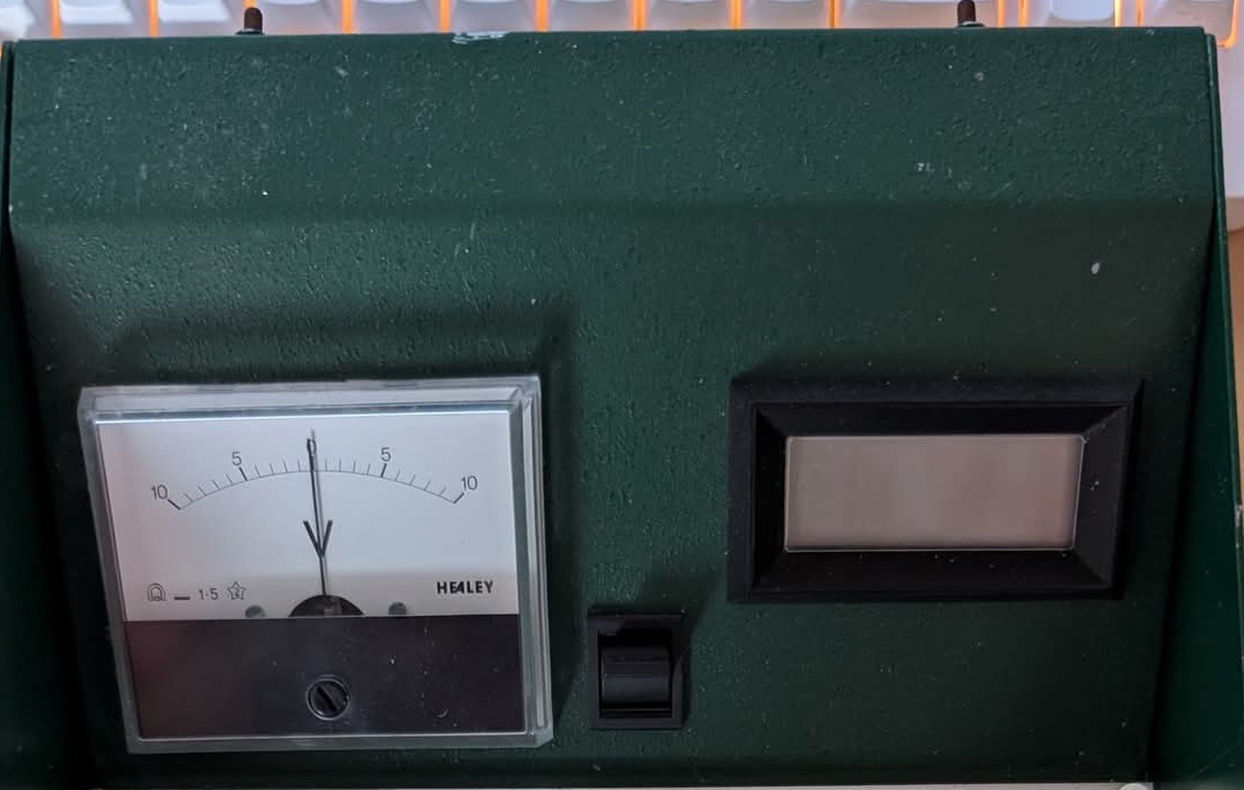
Figure 1 — The upper bezel. Three instruments and one control: the analogue meter, the mode toggle, and an LCD numeric display that is unlit in every held photograph. Crop of a locally held photograph.
2.1 About this Volume
Volume 1 established what the machine is and how thin its documentary record is. This volume describes the console itself: its physical form, the three instruments on its bezel, the geometry of its patch field, and the arrangement by which the field documents the machine behind it.
The central subject here is a design decision rather than a component. On this machine the patch field is not labelled — it is drawn. Each computing element appears as a small circuit diagram with its jacks placed at the electrically meaningful points and its component values printed beside the components they belong to. That decision is why Volumes 3 and 5 can state this machine’s computing complement and arithmetic with confidence despite the total absence of a manual, and it is worth examining as engineering rather than as graphic design.
Cross-references: Vol 1 for the record and its limits; Vol 3 for the elements catalogued one by one; Vol 4 for what lies behind the panel; Vol 6 for the modes and the readout.
2.2 The Physical Machine
The Aeon is a single self-contained desk instrument in a sheet-metal enclosure finished in dark green. The enclosure is a wedge: a tall, near-vertical upper bezel at the back, falling forward to a shallow sloped face that carries the patch field, with the coefficient dials projecting from the front edge below it.
No dimension can be given. None of the three photographs contains a scale object or a ruler, and no dimensional information is printed on the machine. Statements elsewhere about this machine’s size would need a source this series does not have. What the photographs do establish is proportion: the machine is distinctly taller than it is wide, and it is a one-person, one-desk object rather than a rack or console installation.
Three features of the construction are visible and worth recording:
- The patch field is a removable panel. Four white plastic fasteners, one at each corner of the printed overlay, retain it. Photographs 2 and 3 exist because that panel can be released and lifted away, which is also how the machine is serviced.
- The field is hinged rather than merely loose. In photograph 3 the jack board is standing up and leaning back, still tethered to the machine by its wiring harness, rather than lying separated beside it.
- A metal bar spans the front edge beneath the coefficient dials. It reads as either a carrying handle or a tilt stand; the photographs do not settle which, and no legend names it.
2.3 The Upper Bezel
Everything that is not patched lives on the bezel: two indicating instruments and the single control that runs the machine.
2.3.1 The Analogue Meter
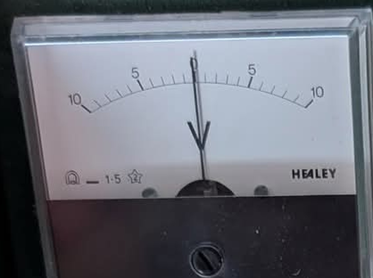
Figure 2 — The analogue meter. The scale is centre-zero, 10–5–0–5–10, matching the machine’s ±10 V signal range directly and without a multiplier. The markings at the lower left are the instrument’s own class symbols; the name at the lower right is the meter’s maker, not the machine’s. Crop of a locally held photograph.
The meter is a moving-coil instrument with a centre-zero scale reading 10–5–0–5–10. Its dial carries the name HEALEY, which is the meter manufacturer — panel meters are bought-in parts, and this name says nothing about who built the Aeon.
Two details of the dial are worth reading carefully, because they are the only performance figures anywhere on this machine:
- The symbols at the lower left include the figure 1·5, which in the standard panel-meter convention denotes an accuracy class of 1.5 per cent of full-scale deflection. On a ±10 V scale that is ±0.15 V.
- The accompanying symbols are the conventional marks for a moving-coil instrument with a permanent magnet, direct current, and a specified insulation test voltage.
This matters more than it first appears. The meter’s class is a property of the meter, not of the computer — but it is nonetheless a hard ceiling on what can be read off the panel by eye. A machine whose only analogue readout is a 1.5 per cent instrument is not a machine on which three-figure answers are taken from the needle. Vol 6 returns to this, and to the likelihood that the digital display exists precisely to get past it.
2.3.2 The Mode Toggle
Between the two displays sits a small black lever-type toggle. It carries no legend of its own; its legend is printed on the patch overlay immediately below, reading ▲RESET — HOLD ▼RUN.
The up-triangle, dash and down-triangle correspond to the three positions of a centre-off lever: up for RESET, centre for HOLD, down for RUN. This is the machine’s entire operating control — there is no separate compute-time control, no repetitive-operation rate knob, and no run-duration timer visible anywhere on the console. Vol 6 treats the consequences.
2.3.3 The Digital Display
At the right of the bezel is a rectangular window containing an LCD numeric panel meter in a black bezel. It is unlit in all three photographs, the machine being unpowered, so neither its digit count nor its decimal-point arrangement can be read.
Its function is therefore genuinely unknown. Nothing on the console labels it, no legend points to it, and no held source describes it. The METER 1 and METER 2 jacks in the right-hand column are the obvious candidates for feeding it, which would make it a patchable digital voltmeter for reading any point in a problem to more figures than the analogue meter allows — but that is a reading of adjacency, not a documented connection. It is listed among the open questions in Vol 7.
2.4 The Patch Field as a Document
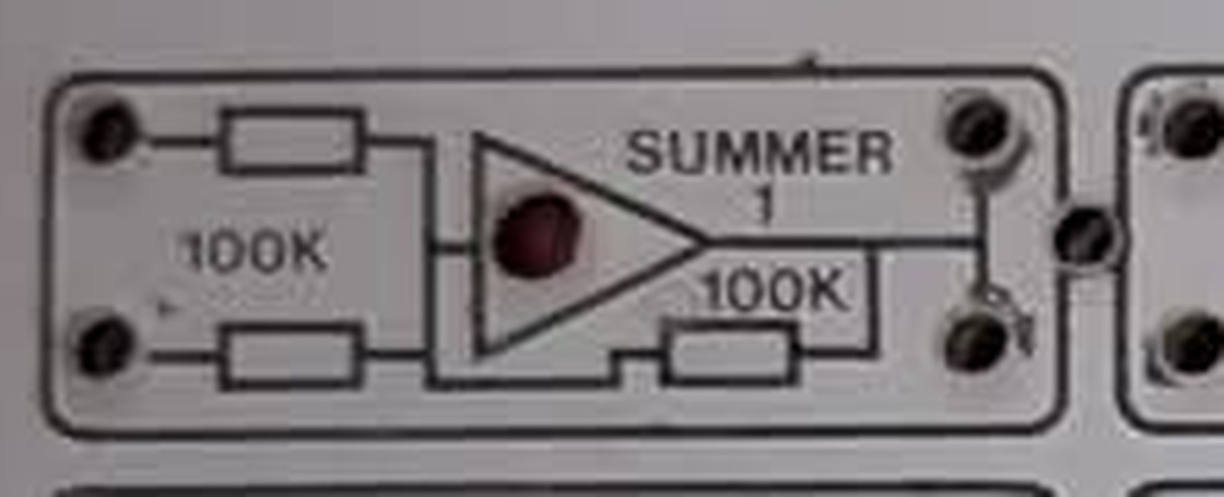
Figure 3 — One element, at magnification. This is not a labelled block: it is a circuit diagram with jacks in it. The two input resistors, the amplifier, the indicator lamp and the feedback resistor are all drawn, and every value is printed. Crop of a locally held photograph.
2.4.1 What the Convention Is
The usual arrangement on a patch-programmed analogue computer is a field of holes with terse labels beside them, and a manual that explains what the labels mean. The Aeon does something else. Each element is printed as a schematic fragment, and the jacks are positioned within that schematic at the points they connect to.
Figure 3 shows the whole idea in one element. Summer 1 is drawn as two resistors, an amplifier symbol and a feedback resistor. The jacks at the far left sit at the free ends of the two input resistors. The jacks at the right sit on the output node. The values 100K and 100K are printed beside the components they describe. An operator who can read that fragment knows, without any manual, that this element inverts, that it sums two inputs, that each input carries unity weight because the feedback resistor equals the input resistors, and precisely which hole each patch cord goes into.
2.4.2 What It Guarantees
The property this buys is that the machine’s functional documentation cannot be separated from the machine. It is silkscreened onto a panel bolted to the front of the hardware it describes. That is why Vol 1 could state this machine’s complete computing complement, every input and feedback value, the reference voltages and the mode scheme, from a single photograph, at a confidence normally requiring a manual.
It is also a teaching decision. A student patching this machine is obliged to look at a circuit diagram of an inverting amplifier every time a cord is moved. The thing being taught is printed on the instrument doing the teaching, and cannot be skipped.
2.4.3 What It Cannot Do
The limits are as sharp as the benefits, and they define the boundary of this series.
A printed legend can state topology and component values. It cannot state tolerance, and this panel does not: no resistor or capacitor on the field carries a tolerance figure, so the accuracy of the machine’s arithmetic is unknown. It cannot state dynamic behaviour: no bandwidth, slew rate, drift or offset figure appears anywhere. It cannot name the active devices: the amplifier is a triangle, not a part number. And it cannot explain why — most sharply, it cannot explain why only two of the six integrators have an initial-condition input, a fact the panel states plainly and accounts for not at all.
2.5 The Geometry of the Field
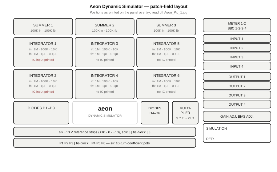
Figure 4 — Map of the patch field, drawn from the positions printed on the panel overlay. Diagram authored for this dive; see photo_credits.txt.
The field is organised in bands, read top to bottom:
Table 1 — The field is organised in bands, read top to bottom
| Band | Contents |
|---|---|
| Summer row | SUMMER 1, SUMMER 2, SUMMER 3, left to right |
| Integrator row 1 | INTEGRATOR 1, INTEGRATOR 3, INTEGRATOR 5 |
| Integrator row 2 | INTEGRATOR 2, INTEGRATOR 4, INTEGRATOR 6 |
| Non-linear row | diodes D1–D3, the wordmark, diodes D4–D6, the multiplier |
| Reference row | six ±10 V strips with a tie block between two groups of three |
| Potentiometer row | P1 P2 P3, a tie block, P4 P5 P6 |
Two features of this arrangement are deliberate enough to be worth naming.
The integrators are numbered down the columns, not across the rows. Integrators 1 and 2 sit one above the other at the left; 3 and 4 in the centre; 5 and 6 at the right. The machine is therefore laid out as three vertical pairs of integrators, not as two horizontal rows of three. Since a second-order differential equation requires exactly two integrators in cascade, this is the natural physical grouping for the commonest problem the machine will ever be asked to solve, and it places each such pair side by side under the operator’s hand. The fact that the pair carrying the initial-condition inputs is the pair numbered 1 and 2 fits the same logic, though as Vol 6 notes, whether that is design or coincidence cannot be established from the photographs.
The field is mirrored about a central spine. The reference and potentiometer rows both run three elements, then a tie block, then three elements. The tie blocks — groups of three jacks joined by a printed line, providing paralleled common points with no component in them — sit at the centre of the field where a patch cord from either half can reach them.
2.5.1 The Jacks
The jacks themselves are small sockets taking a pin-type patch cord rather than a full-size banana plug. Within the computing elements they are uniform in size. In the right-hand input and output rows they are not: each of those rows carries a mixture of two visibly different socket diameters, two smaller and two larger. No legend explains the mixture, and the reason for it — different plug standards for different classes of connection, most plausibly — is not established by anything held here.
2.6 The Host-Computer Column
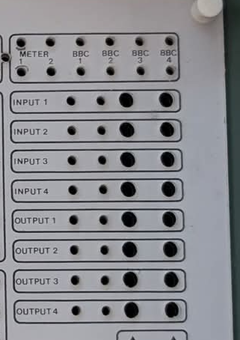
Figure 5 — The interface column. Four BBC channels, four INPUT rows, four OUTPUT rows and two METER positions. Crop of a locally held photograph.
Down the right-hand side of the field, separated from the computing elements, runs a column of jacks that is not a computing element at all:
Table 2 — Down the right-hand side of the field, separated from the computing elements, runs a column of jacks that is not a computing element at all
| Group | Positions |
|---|---|
METER | 1, 2 |
BBC | 1, 2, 3, 4 |
INPUT | 1, 2, 3, 4 |
OUTPUT | 1, 2, 3, 4 |
This is an interface to something outside the machine, and its presence is one of the strongest statements the console makes about what the Aeon was for.
The BBC reading. In a British teaching instrument of the late 1980s — and Vol 1 sets out the evidence for British origin and that date — “BBC” denotes the BBC Microcomputer, the standard computer of British schools in that period. The BBC Micro’s analogue port provides exactly four analogue input channels, which matches BBC 1–BBC 4 precisely. On that reading the column is a pre-wired harness point for feeding four of the machine’s problem variables to a BBC Micro for digital capture, plotting or logging.
This is the most economical explanation of four jacks so labelled on a machine of this type and date, and it is the reading this series adopts. It is nonetheless an inference. No held source confirms it, no cable or interface box accompanies the machine, and the electrical arrangement behind those jacks — whether buffered, attenuated to the BBC’s 0–1.8 V input range, or passed straight through at ±10 V — cannot be determined from the photographs. That last point is not academic: the BBC Micro’s analogue input will not tolerate ±10 V directly, so some conditioning must exist somewhere, and where it exists is unknown.
The INPUT and OUTPUT rows are the general case of the same idea: four channels in and four channels out, patchable to any point in a problem, available for a recorder, an oscilloscope, a signal source or the host machine.
2.7 The Operator’s Annotations
Two features of the field exist for the person using the machine rather than for the mathematics.
The SIMULATION / REF: box is a blank rectangle printed on the field with those two words in it and nothing else — a write-on area for naming the problem currently patched and giving a reference to wherever it is written up. Its presence implies a working pattern in which a problem is patched, labelled, and left standing: the next class, or the next session, finds the machine already set up and can see what it is set up for.
GAIN ADJ. and BIAS ADJ. are two access holes, each marked with a triangle, giving a screwdriver at trimmers behind the panel. Bringing two adjustments to the front of the machine while leaving the rest of the machine’s trimmers inside implies these two are expected to be touched in normal use rather than at service intervals. Vol 6 discusses what they most plausibly adjust and marks the discussion as reconstruction.
2.8 What the Console Design Buys, and What It Costs
What it buys. The machine explains itself. Its documentation is physically attached, cannot be lost, cannot go out of date, and is exactly as detailed as an operator needs to patch a problem correctly. For a teaching instrument this is close to ideal, and it is the reason a machine whose every scrap of paperwork has vanished can still be catalogued in detail sixty pages further on.
What it costs. Three things.
The complement is frozen. Nothing plugs in. Where the TR-10’s capability is decided by which modules are in the cupboard, the Aeon has three summers and six integrators permanently, because they are etched onto a board and drawn onto a panel. A problem needing a seventh integrator needs a second machine.
The program is not portable. The patch field is the machine’s own front panel, not a removable problem board. A patched problem cannot be lifted out and stored; re-running last term’s problem means patching it again. The SIMULATION / REF: box is the designer’s mitigation for exactly this — write down what it is, and where the working is.
The documentation stops at the panel. Everything the legend states is trustworthy and everything it omits is simply gone. There is no second layer to fall back on. A machine documented only on its own face is documented only as far as its face goes, which is why Vol 4 reaches a hard boundary the moment the question becomes what the circuit actually does.
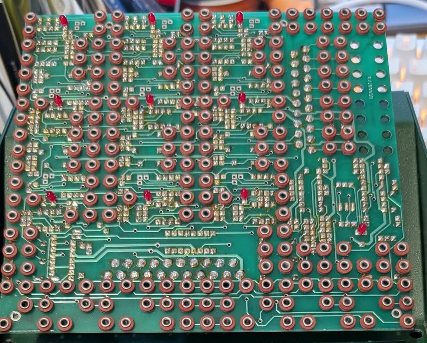
Figure 6 — The patch field from behind, lifted away from the machine. The field is a printed-circuit board carrying the socket bodies; the printed overlay is on its outer face. Crop of a locally held photograph.
2.9 What Comes Next
Vol 3 takes the computing elements one at a time — summers, integrators, coefficient potentiometers, diodes, the multiplier, the reference strips and the tie blocks — with the values printed beside each and a census of the whole field. Vol 4 goes behind the panel photographed in Figure 6, to the board stack and the semiconductor complement. Vol 5 turns the printed values into arithmetic and works a problem onto the machine. Vol 6 returns to the bezel instruments and the mode lever, and reconstructs an operating and calibration sequence.
Comments (0)