Aeon Dynamic Simulator · Volume 3
Aeon Dynamic Simulator — Volume 3 — The computing elements
Every element on the patch field catalogued from its printed legend: three summers, six integrators, six coefficient potentiometers, six diodes, a multiplier, the reference strips and the tie blocks
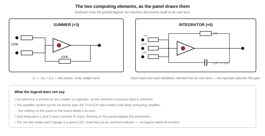
Figure 1 — The machine’s two amplifier-based elements, redrawn from the printed legend. Diagram authored for this dive; see photo_credits.txt.
3.1 About this Volume
This volume catalogues every computing element on the Aeon’s patch field, one class at a time, stating for each what the printed legend says and what it does not.
The discipline throughout is that of Vol 1: the panel is the only source. Where a value is printed, it is quoted. Where a value is absent — and the most important ones are — that absence is recorded rather than filled from general knowledge of comparable machines. There is no manual to check any of this against.
Cross-references: Vol 2 for the field’s geometry and the interface column; Vol 4 for the hardware behind the panel; Vol 5 for the arithmetic these elements perform; Vol 6 for modes and readout.
3.2 The Element Census
Counted directly from the legend in the held photograph of the closed machine:
Table 1 — Counted directly from the legend in the held photograph of the closed machine
| Element | Count | Designators | Printed values |
|---|---|---|---|
| Summer | 3 | SUMMER 1–3 | 100 kΩ inputs (2 each), 100 kΩ feedback |
| Integrator | 6 | INTEGRATOR 1–6 | inputs 1 MΩ, 100 kΩ, 10 kΩ (two each); feedback 1 MΩ, 1 µF, 0·1 µF |
| Coefficient potentiometer | 6 | P1–P6 | none printed |
| Diode | 6 | D1–D6 | none printed |
| Multiplier | 1 | unlabelled block | inputs X, Y, Z; one OUT |
| Reference strip | 6 | unlabelled | +10 / 0 / −10 |
| Tie block | 2 | unlabelled | three paralleled jacks each |
The amplifier count is therefore nine — three summers and six integrators. That happens to be the same number of amplifiers as the Heathkit EC-1 of thirty years earlier, a coincidence Vol 7 returns to.
3.3 The Summers
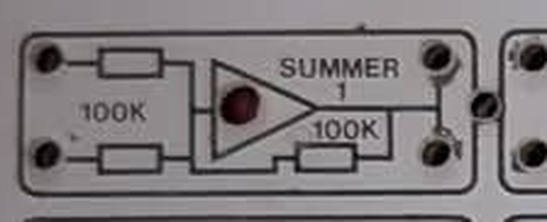
Figure 2 — Summer 1. Crop of a locally held photograph.
3.3.1 What the Legend States
Each of the three summers is drawn as:
- Two input resistors, both marked
100K, each terminating in its own jack at the left edge of the block. - An amplifier symbol — a triangle, apex right — containing a red indicator lamp.
- One feedback resistor, marked
100K, drawn from the output back to the amplifier’s input node. - Output jacks at the right, joined by a printed line indicating that they are paralleled.
3.3.2 What Follows From It
Because the feedback resistor and both input resistors are the same value, each input carries unity weight, and the element computes
eₒ = −(e₁ + e₂)
The inversion is not optional and is not a defect: it is inherent to the operational-amplifier summing circuit, and it is the single most important thing a programmer of this machine has to keep track of. Vol 5 treats sign management as a programming discipline, because with only nine amplifiers available, an inverter spent purely on correcting a sign is an inverter not spent on the problem.
There is no third input, and no provision for a different input weight. A summer on this machine adds exactly two things, each with weight one. Weighted sums must be built by feeding a summer through the coefficient potentiometers, or by using an integrator’s 1 MΩ feedback resistor as described below.
3.3.3 What the Legend Does Not State
No tolerance for either resistor; no device type for the amplifier; no stated function for the indicator lamp, though Vol 4 shows a comparator beside every amplifier group on the board, which is what an overload detector looks like.
3.4 The Integrators
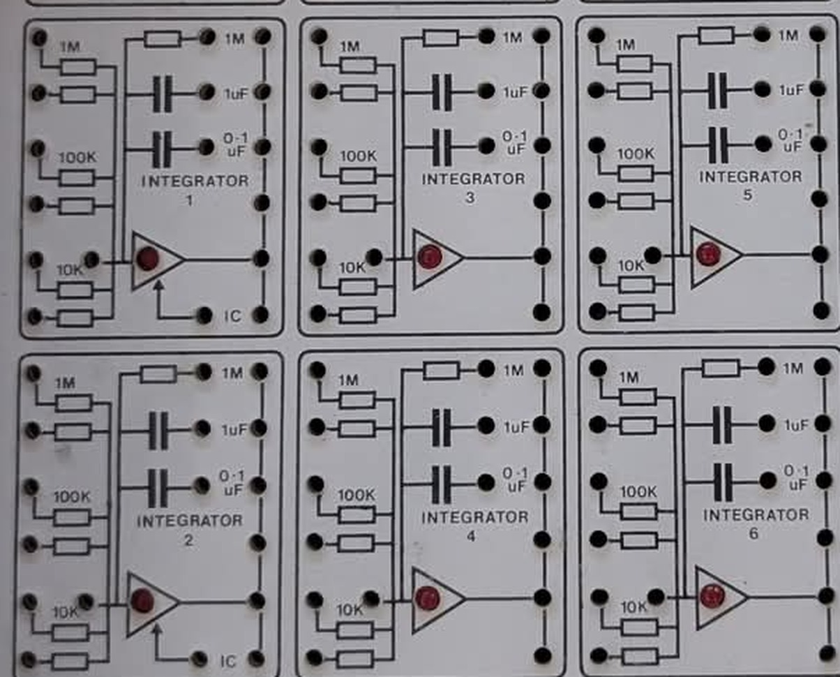
Figure 3 — All six integrators. Crop of a locally held photograph.
The integrators are the most capable elements on the machine and the most generously provided with patching options.
3.4.1 Inputs
Each integrator has six input jacks, arranged as three pairs, each pair sharing a printed value:
Table 2 — Each integrator has six input jacks, arranged as three pairs, each pair sharing a printed value
| Pair | Value |
|---|---|
| Upper | 1 MΩ |
| Middle | 100 kΩ |
| Lower | 10 kΩ |
Each jack terminates its own resistor, so all six may be used at once. Two inputs at each of three decades gives the programmer a choice of input weight spanning a hundred to one without touching a component — the weight is selected by which hole the cord goes into. This is the feature that makes the machine genuinely flexible despite its fixed complement.
3.4.2 Feedback
Three feedback elements are provided, each with its own jack:
Table 3 — Three feedback elements are provided, each with its own jack
| Element | Value | Effect when patched |
|---|---|---|
| Resistor | 1 MΩ | the element becomes a summer |
| Capacitor | 1 µF | integration, larger time constant |
| Capacitor | 0·1 µF | integration, smaller time constant |
The resistor is the important one and is easy to overlook. Patching the 1 MΩ feedback resistor instead of a capacitor converts an integrator into an inverting amplifier of gain −1, −10 or −100, depending on which input resistor is used. The machine therefore does not really have three summers and six integrators; it has three summers and six elements that are each an integrator or a summer at the operator’s choice. Vol 5 works through what that does to the machine’s effective capacity.
3.4.3 The Initial-Condition Asymmetry
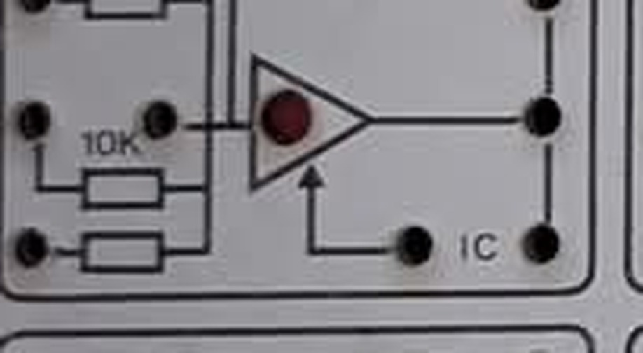
Figure 4 — Integrator 1. An arrow runs from a dedicated jack into the amplifier, and the jack is labelled IC. Crop of a locally held photograph.
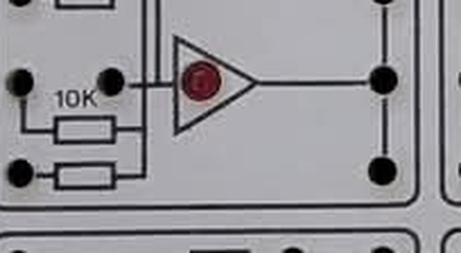
Figure 5 — Integrator 3, at identical magnification and framing. The arrow and the IC legend are simply absent. Crop of a locally held photograph.
Integrators 1 and 2 carry a printed initial-condition input: a dedicated jack labelled IC, with an arrow running from it into the amplifier. Integrators 3, 4, 5 and 6 do not. Every other feature of all six blocks — input resistors, feedback options, output jacks, indicator lamp — is identical.
Figures 4 and 5 are reproduced at the same magnification and framing precisely so that the difference can be checked rather than taken on trust. This is not a printing fault on one machine, and it is not an artefact of the photograph: the legend is absent on four elements and present on two.
The consequence is severe and is the single most important practical fact about programming this machine. An integrator is a device for solving a differential equation, and a differential equation without an initial condition has no particular solution. On this machine, only two of the six integrators can be given a patchable non-zero starting value. The other four necessarily start from whatever RESET leaves them at, which for a capacitor shorted or driven to zero is zero.
Two readings are available and the held sources do not decide between them:
- It is deliberate and sufficient. A second-order problem needs exactly two initial conditions, and a second-order problem is what a teaching machine solves most of the time. Providing IC inputs on one integrator pair and not on the others is then an economy, not an omission — and the pair chosen is the pair numbered 1 and 2, which Vol 2 notes sit one above the other as the leftmost vertical pair.
- The others have initial-condition circuitry that is simply not brought to the panel. The board carries switching devices at every amplifier group, not only at two of them (Vol 4), so the hardware for resetting all six exists. What is absent is a patchable way to set a non-zero value on four of them.
Nothing held here settles it. What can be said without inference is that the panel offers a patchable initial condition on two integrators and not on four, and that any problem needing three or more independent non-zero initial conditions cannot be set up on this machine as it is drawn.
3.5 The Coefficient Potentiometers
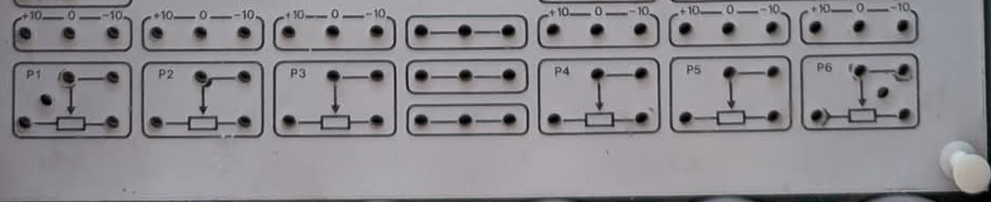
Figure 6 — The reference and potentiometer rows. Crop of a locally held photograph.
Six coefficient potentiometers, P1 through P6, occupy the lowest band of the field, with their ten-turn counting dials projecting from the front edge of the machine below the panel.
Each is drawn on the legend as a resistor with a wiper arrow descending into it. The jacks are placed so that:
- the two ends of the track terminate in the two lower jacks of the block, and
- the wiper terminates in the upper jacks, which are joined by a printed line and therefore paralleled.
The significant point is that both ends of the track are patchable. The pots are not internally grounded at one end, as coefficient pots on simpler machines often are. An ungrounded pot can be patched as a divider between any two voltages in the problem — between a reference strip and ground for a conventional coefficient between 0 and 1, but equally between +10 V and −10 V to produce a coefficient continuously variable from −1 through 0 to +1, which is exactly what setting a damping term or a sign-ambiguous parameter requires.
Ten turns of dial across that range gives fine resolution by hand. The counting dials allow a coefficient to be recorded and returned to, which is what makes the SIMULATION / REF: box of Vol 2 useful.
No resistance value is printed for the potentiometers anywhere on the panel. This is a real gap. The pot’s track resistance determines how heavily it loads the source driving it and how heavily it is loaded by whatever it drives, and therefore how far the dial reading departs from the coefficient actually delivered. Without that value, the loading error cannot be estimated. The trimmers visible inside the machine are marked, but they are trimmers, not the panel pots, and their values cannot be transferred to the panel pots by assumption.
3.6 The Diodes
Six diodes, D1, D2 and D3 in a block at the left of the non-linear row and D4, D5 and D6 in a block to the right of the wordmark. Each is drawn as a single diode symbol between two jacks, with the cathode bar marked, so its orientation in a patch is unambiguous.
They carry no type number and no specification — no forward voltage, no current rating, no indication of whether they are silicon signal diodes, germanium, or something selected for a low and repeatable forward drop.
A patchable diode is the basic non-linear building block of an analogue computer, and six of them with both ends free is a generous provision on a machine this size. With an amplifier and a reference voltage a diode gives a limiter or a bounded output; two in opposition give a dead zone; a diode across an amplifier’s feedback path gives a half-wave rectifier, and two arranged around one give absolute value; diodes with different reference voltages in parallel give a piecewise-linear function generator approximating an arbitrary curve.
That last construction deserves note, because the Aeon has no dedicated function generator — no diode function generator module, no log or squaring element. The six diodes are the entire non-linear provision apart from the multiplier, and building a curve out of them consumes both diodes and amplifiers from a total of nine.
3.7 The Multiplier
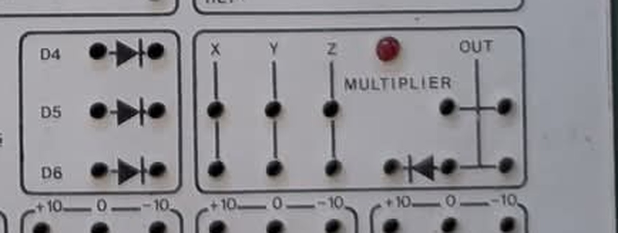
Figure 7 — The diode block and the multiplier. Crop of a locally held photograph.
One multiplier block is provided. Its legend shows:
- three inputs labelled
X,YandZ, each with a pair of paralleled jacks; - an output labelled
OUT; - a red indicator lamp;
- an additional diode symbol inside the block, unlabelled, positioned near the output.
The X, Y, Z labelling is the conventional pin nomenclature of the integrated-circuit analogue multipliers of the period, in which the device forms a product of two inputs and a third terminal provides a summing or denominator connection — the arrangement that lets one part serve as a multiplier, a divider, a squarer or a square-root element depending on how it is patched. On that reading the Aeon’s single block provides all four of those functions.
This is, however, an inference from a labelling convention. No device type is printed on the panel, no multiplier IC could be positively identified in the interior photographs, and the block’s internal arrangement is not drawn on the legend in the way the summers and integrators are — the multiplier is the one element the panel presents as a black box. What the multiplier’s accuracy is, what its input and output ranges are, and whether division is actually supported are all unknown.
The unlabelled diode inside the block is unexplained. It is a seventh diode symbol on a panel that labels exactly six, and the interior photographs show board designators running to at least D8. Whether it is a patchable element in its own right, a clamp belonging to the multiplier circuit, or part of a square-root configuration cannot be determined from the legend.
3.8 The Reference Strips and Tie Blocks
Six reference strips run across the field above the potentiometer row, each printed +10 — 0 — −10 with three jacks. These are the machine’s unity: every coefficient set on a pot, every initial condition and every constant term in a problem is ultimately a fraction of this voltage. Six of them, distributed across the width of the field, means a reference connection is always within short patch-cord reach of wherever it is needed, and the count corresponds to the six potentiometers each requiring a supply.
Their accuracy is unknown. No tolerance or stability figure is printed, and since the whole machine’s arithmetic is scaled to this voltage, that omission propagates to everything. Vol 4 notes the +10 and −10 test points on the lower board, which is where a calibration procedure would begin.
Two tie blocks, one in the reference row and one in the potentiometer row, each provide three jacks joined by a printed line and containing no component. They are common points — somewhere to join several cords, or to park one. Their placement at the centre of the field, between the two groups of three, puts them within reach from either half.
3.9 The Indicator Lamps
A red lamp is drawn inside the amplifier triangle of every summer and every integrator — nine in all — and a tenth inside the multiplier block. Nothing on the panel states what they indicate.
The reading adopted here, and flagged as a reading, is that they are overload indicators. Vol 4 shows an LM393P comparator sitting beside the computing amplifier in each group on the board, and board silkscreen running LED1 through at least LED10. A comparator per amplifier driving a lamp per amplifier is what overload detection looks like, and overload detection is the single most valuable diagnostic an analogue computer can offer: an amplifier driven past its supply rails stops obeying the equation, and goes on producing a smooth, plausible and completely wrong curve. A lamp converts that silent failure into a visible one and identifies which element to rescale.
3.10 What the Element Set Can and Cannot Do
What it can do. Nine amplifiers, six of them convertible between integration and summing, with input weights spanning two decades selected by patch position, six ungrounded coefficient pots, six diodes and a multiplier. That supports linear systems up to a useful order, second- and third-order non-linear problems, and the standard teaching repertoire: damped oscillators, coupled masses, predator–prey systems, simple flight and vehicle dynamics, chemical kinetics.
What it cannot do. The limits are worth stating as plainly as the capabilities:
- No dedicated function generator. Arbitrary non-linear functions must be built from the six diodes at a cost in amplifiers.
- No comparator or relay brought to the panel. There is no patchable element for switching behaviour on a threshold — the bouncing-ball and hysteresis problems that a machine with a comparator handles directly are awkward here.
- No track-store or memory element.
- No more than two patchable non-zero initial conditions, as set out above.
- A fixed complement. Nothing plugs in; a problem needing a tenth amplifier needs a second machine.
3.11 What Comes Next
Vol 4 goes behind the panel to the board stack, reads the semiconductor complement off the interior photographs, and marks precisely where the absence of a schematic stops the analysis. Vol 5 turns the values catalogued here into the machine’s arithmetic and works a second-order problem onto the hardware. Vol 6 covers the mode lever, the initial-condition arrangement in operation, readout and a reconstructed calibration sequence.
Comments (0)