Aeon Dynamic Simulator — Volume 5 — Programming and scaling

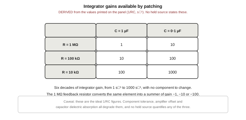
Figure 1 — The integrator gains the printed values make available. Derived for this dive from the panel legend; no held source states them. Diagram authored for this dive.

5.1 About this Volume

This volume turns the component values catalogued in Vol 3 into the machine’s arithmetic, and then works two problems onto it.

Everything in this volume is derived. No held source states a single one of the results below — there is no manual, no worked-example booklet and no teaching notes for this machine. What the panel provides is component values; what follows from them is ordinary operational-amplifier theory, applied here and shown in full so that each step can be checked. Where a derivation depends on something the panel does not state, that dependency is named.

Cross-references: Vol 3 for the elements and their printed values; Vol 6 for modes, initial conditions and readout; Vol 4 for what is known of the hardware.

---

5.2 The Machine Unit

Every analogue computer has a voltage that represents unity, and on this machine it is 10 V. The six reference strips are each printed +10 — 0 — −10; the panel meter is a centre-zero instrument scaled 10–5–0–5–10; the lower board carries test points labelled +10 and −10.

A problem variable is therefore represented as a fraction of 10 V, and the programmer’s first task is always the same: choose, for each variable, a scale factor relating the variable’s real-world units to machine volts, such that the variable’s largest excursion during the run approaches but does not exceed 10 V.

Two consequences follow immediately.

Too small is as bad as too large. A variable scaled so that it never exceeds 0.1 V is using one per cent of the machine’s range, and its answer carries one per cent of the available resolution. Since the analogue meter is a 1.5 per cent instrument (Vol 2), a signal of 0.1 V is entirely below the noise of the readout.

Too large is worse. An amplifier driven beyond its supply rails stops obeying its equation. It does not announce this: it continues to produce a smooth, plausible curve that is simply wrong. This is the failure mode the indicator lamps exist to catch, and it is why Vol 3 reads the red discs inside the amplifier triangles as overload lamps. The lamps are the scaling feedback loop: patch, run, watch for a lamp, rescale.

---

5.3 The Elements as Arithmetic

5.3.1 The Summer

From Vol 3, each summer has two 100 kΩ inputs and a 100 kΩ feedback resistor:

eₒ = −(e₁ + e₂)

Two inputs, unity weight each, and an inversion. There is no third input and no alternative weight.

5.3.2 The Integrator with a Capacitor

With input resistor R and feedback capacitor C:

eₒ = −(1 / RC) ∫ eᵢ dt

The quantity k = 1/RC is the integrator gain, in reciprocal seconds. Because the integrator’s summing junction accepts all six of its input jacks at once, an integrator also sums — and it can sum inputs at different gains simultaneously, since each input jack has its own resistor.

5.3.3 The Integrator with the 1 MΩ Feedback Resistor

Patching the 1 MΩ feedback resistor instead of a capacitor makes the element an inverting amplifier:

eₒ = −(Rf / Rᵢ) eᵢ

giving gains of −1, −10 and −100 from the 1 MΩ, 100 kΩ and 10 kΩ input resistors respectively. This is why Vol 3 insists the machine has six elements that are either integrator or summer, not six integrators.

Note what this buys that the dedicated summers do not offer: a weighted sum. The three SUMMER elements add with unity weight only; an integrator in resistor-feedback mode can add with weights of 1, 10 and 100 in any combination across its six inputs.

5.3.4 The Coefficient Potentiometer

A pot sets a coefficient between 0 and 1 when patched between a reference and ground. Because both track ends are brought to jacks (Vol 3), patching it across a reference strip from +10 to −10 gives a coefficient continuously variable from −1 through 0 to +1.

The pot introduces no inversion and no gain above unity. It can only attenuate.

---

5.4 The Gain Matrix

Three input resistors and two feedback capacitors give six combinations:

Table 1 — Three input resistors and two feedback capacitors give six combinations

	C = 1 µF	C = 0·1 µF
R = 1 MΩ	1 s⁻¹	10 s⁻¹
R = 100 kΩ	10 s⁻¹	100 s⁻¹
R = 10 kΩ	100 s⁻¹	1000 s⁻¹

Four distinct gains spanning three decades, selected entirely by patch position.

The duplication is useful rather than wasteful. A gain of 10 s⁻¹ is available either as 1 MΩ with 0·1 µF or as 100 kΩ with 1 µF. These are electrically different: the first presents ten times the input impedance, loading the driving element ten times less, which matters when the driving element is a potentiometer whose own resistance is unknown (Vol 3). The second stores ten times the charge, which makes it less sensitive to the amplifier’s input bias current and therefore drifts less on HOLD. A programmer with a loading problem takes the high-resistance route; one with a drift problem takes the high-capacitance route.

Caveat — These are ideal 1/RC figures. Real gain departs from them by the tolerance of the resistor and capacitor, neither of which is printed anywhere on this machine, and by the amplifier’s finite gain and offset, which are equally unknown. No error budget can be constructed for this machine from the sources held.

---

5.5 Time Scaling

The integrator gain k is also the machine’s time-scale factor. An integrator of gain k run for one second of machine time advances the problem by k seconds of problem time if the problem is written in seconds.

The practical question is always the same: how fast should the solution run?

• Too slow, and the operator watches a needle creep for minutes.
• Too fast, and the solution is over before the meter needle has physically moved — the meter is a mechanical instrument with its own response time.

For a solution to be watched on the analogue meter, a run of a few seconds to a few tens of seconds is the useful range. For a solution to be captured by the host computer through the interface column (Vol 2), much faster runs are appropriate, limited by whatever the host can sample.

The machine has no repetitive-operation facility. There is no rate control, no repetitive mode on the lever, and no multivibrator to cycle it — the mode legend reads only RESET, HOLD and RUN. A solution is therefore run once, by hand, and observed or captured once. Machines of the previous generation, such as the Heathkit EC-1, offered a repetitive mode precisely so that a solution could be re-run many times a second and displayed as a stationary trace on an oscilloscope. The Aeon’s designers appear to have expected the host computer to do that job instead, capturing a single run and plotting it. This is an inference from the absence of a control and the presence of an interface, and it is marked as such.

---

5.6 Sign Discipline

Every active element on this machine inverts. The summers invert, the integrators invert, and the pots cannot invert. Sign management is therefore not a detail but the central programming constraint, and on a machine with only nine amplifiers it has a direct cost: an amplifier spent producing a sign change is an amplifier not spent on the problem.

Two rules follow.

Count inversions around every loop. A signal passing through n amplifier elements arrives with sign (−1)ⁿ. A feedback loop must arrive with the sign the equation requires; if it does not, the simulation will either run away or settle to the wrong answer, and it will do so smoothly and convincingly.

Take advantage of the intermediate nodes. A cascade of two integrators produces −ẋ at the first output and +x at the second. Both are available for patching, at no additional cost, and a term needing +ẋ or −x may be obtainable from a node already in the circuit rather than from a new inverter.

---

5.7 A First Worked Problem: Exponential Decay

The simplest problem on the machine, and the right one to patch first when checking that it works.

The equation. ẋ = −λx, with x(0) = x₀.

The patch. One integrator. Its output is fed back through a coefficient potentiometer to one of its own input jacks. The initial condition is applied at the IC jack, which means the integrator must be integrator 1 or integrator 2 — the only two with a printed IC input (Vol 3).

The derivation. Let the integrator have gain k and let the pot be set to a. The integrator’s output v obeys

v = −k ∫ (a v) dt ⟹ v̇ = −k a v

so the decay constant is λ = k a, and v = x₀ e^(−kat).

A setting. With the 100 kΩ input and the 1 µF capacitor, k = 10 s⁻¹. A pot setting of a = 0·5 gives λ = 5 s⁻¹, a time constant of 0·2 s, and a solution essentially complete in about one second. For a leisurely run, the 1 MΩ input with 1 µF gives k = 1 s⁻¹ and a = 0·5 gives a 2-second time constant.

Because this problem has a known closed-form answer, it is also the machine’s self-test: set x₀ to full scale, run, and confirm the output falls to 37 per cent of its initial value in one time constant. A significant discrepancy points at the pot’s loading, the capacitor’s tolerance or the integrator’s gain — and since none of those is specified for this machine, this measurement is the only route to any of them.

---

5.8 The Main Worked Problem: A Damped Second-Order System

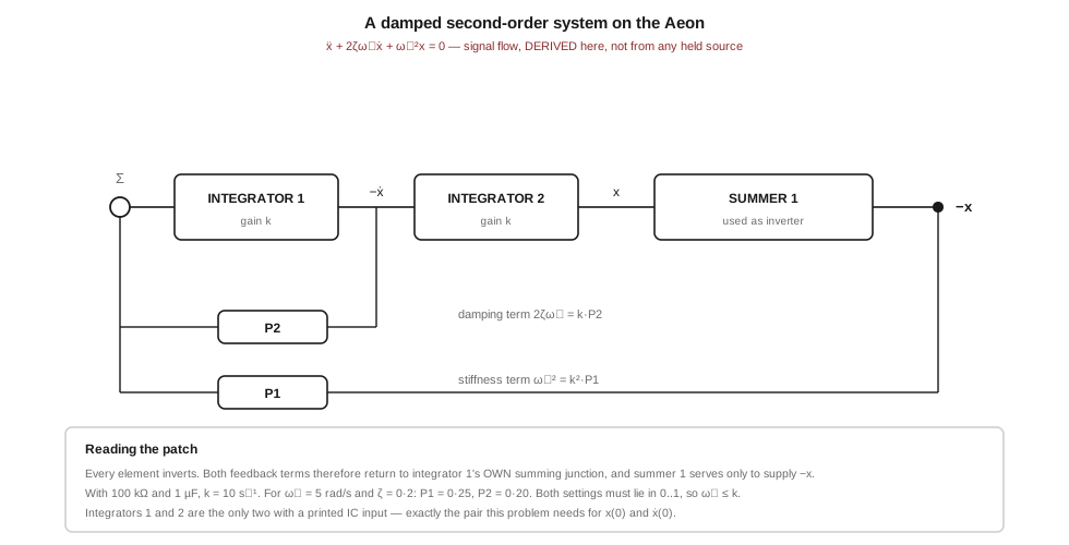
Figure 2 — The damped second-order patch. Derived for this dive; no held source states it. Diagram authored for this dive.

The equation. The standard damped oscillator, covering a mass on a spring with a dashpot, an RLC circuit, a galvanometer movement and a first-cut vehicle suspension:

ẍ + 2ζω_n ẋ + ω_n² x = 0

Why the obvious patch fails. The natural first attempt is to cascade two integrators and close the loop through a summer. That arrangement contains three inversions, and it does not work: solving for the required coefficients yields negative values for the pot settings, and a potentiometer cannot produce a negative coefficient unless it is patched across a reference strip, which changes the scaling of the term it feeds. This is worth stating because the failure is not obvious until the algebra is done, and the resulting circuit looks entirely plausible.

The arrangement that does work. Both feedback terms return to the first integrator’s own summing junction, and the summer is used purely as a unity inverter to supply −x:

Table 2 — The arrangement that does work. Both feedback terms return to the first integrator's own summing junction, and the summer is used purely as a unity inverter to supply −x

Element	Role	Output
Integrator 1	gain k; sums both feedback terms	−ẋ
Integrator 2	gain k	x
Summer 1	used as an inverter, one input	−x
P2	damping coefficient, from integrator 1’s output	—
P1	stiffness coefficient, from summer 1’s output	—

The derivation. Let v₁ be integrator 1’s output and v₂ integrator 2’s output, both integrators having gain k. Integrator 2 takes v₁ alone:

v̇₂ = −k v₁ ⟹ v₁ = −v̇₂ / k

Integrator 1 sums its own output through P2 (setting α) and the inverter’s output −v₂ through P1 (setting β):

v̇₁ = −k ( α v₁ + β (−v₂) ) = −k α v₁ + k β v₂

Substituting v₁ = −v̇₂/k:

−v̈₂ / k = α v̇₂ + k β v₂

v̈₂ + k α v̇₂ + k² β v₂ = 0

Comparing term by term with the target equation, and identifying v₂ with x:

2ζω_n = k · P2 and ω_n² = k² · P1

Setting the pots. Inverting those two relations:

P1 = (ω_n / k)² and P2 = 2ζω_n / k

Take the 100 kΩ inputs with 1 µF capacitors, so k = 10 s⁻¹, and a problem with ω_n = 5 rad/s and ζ = 0·2:

P1 = (5/10)² = 0·25 P2 = 2(0·2)(5)/10 = 0·20

Both lie comfortably within the pots’ 0-to-1 range, and both are settable to three figures on a ten-turn counting dial.

The range constraint. Since P1 and P2 must lie between 0 and 1, the patch requires ω_n ≤ k and 2ζω_n ≤ k. If the problem’s natural frequency exceeds the integrator gain, the remedy is to move to a faster gain from the matrix above — which is time scaling, arrived at from the other direction.

Initial conditions. A second-order problem needs two: x(0) and ẋ(0). They are applied at the IC jacks of the two integrators. This patch therefore requires integrators 1 and 2 specifically, because they are the only two the panel provides with an IC input. That the machine’s one pair of IC-equipped integrators is exactly what its commonest problem requires is noted in Vol 3 as suggestive; whether it is design or coincidence remains unresolved.

Running it. Set P1 and P2; set the two initial conditions; hold the lever at RESET; move to RUN and watch. With ω_n = 5 rad/s the oscillation has a period of about 1·3 seconds and, at ζ = 0·2, decays to negligible amplitude in roughly four seconds — slow enough for the meter needle to follow, and a good match to the machine’s unaided readout.

Checking it. The damped period should be 2π/(ω_n√(1−ζ²)), and successive peaks should fall in constant ratio. Both are measurable at the output, and both are derivable in closed form, so this problem doubles as a calibration check on the integrator gains and the pot settings together.

---

5.9 Using the Non-Linear Elements

The six diodes and the multiplier extend the repertoire beyond linear systems, at a cost in amplifiers.

A limiter is the commonest construction: a diode patched from an amplifier’s output to a reference-derived voltage clamps the output at that voltage, turning the linear second-order system above into one with a mechanical stop. A pair of diodes in opposition around one amplifier gives a dead zone, which is how backlash and static friction enter a mechanical simulation. Two diodes arranged around an amplifier give absolute value, and several diodes with different reference voltages give a piecewise-linear approximation to an arbitrary curve.

The multiplier supplies the genuinely non-linear products — a term in x², or xy for a predator–prey system, or a velocity-squared drag term. As Vol 3 records, the multiplier is the one element the panel presents as a black box: its accuracy, its input range and whether it also divides are all unknown, so any problem depending on it should be checked against a case with a known answer before its results are trusted.

---

5.10 Where the Arithmetic Stops

Everything above follows from the values printed on the panel by ordinary operational-amplifier theory. What cannot be established is how good any of it is:

• No error budget. No tolerance is printed for any resistor or capacitor, so no gain is known better than “nominal”.
• No loading correction. The potentiometers’ track resistance is not stated, so the departure of a dial reading from the coefficient actually delivered cannot be estimated.
• No drift figure. The rate at which an integrator’s output moves on HOLD, with nothing patched to its input, is the figure that limits how long a solution can be paused. It is unknown.
• No bandwidth figure. The highest integrator gain in the matrix, 1000 s⁻¹, may or may not be usable at full amplitude; the amplifier’s slew rate and bandwidth are unstated.

The only route to any of these numbers is measurement on a working machine, starting from the exponential-decay test above and the +10/−10 test points identified in Vol 4.

---

5.11 What Comes Next

Vol 6 covers operating the machine: the three-position lever, what RESET, HOLD and RUN do and where the initial-condition asymmetry bites in practice, the two readout instruments, the overload lamps, and a reconstructed calibration sequence built on the test points. Vol 7 places the machine among its contemporaries and sets out every inference this series has made, with the confidence attaching to each.